


1. Introduction
Non-Brownian suspensions are widespread in industry (paints, fresh concrete, solid rocket propellants, etc.) as well as in biological (blood) and natural (mud, lava, submarine avalanche, etc.) flows, to mention but a few. This widespread presence of suspensions has encouraged active research in the past years that has revealed great complexity in the behaviour of these systems. Even the simplest suspensions, non-Brownian suspensions made of rigid single-sized spherical particles suspended in a Newtonian fluid and sheared in a viscous creeping flow, can exhibit a rich variety of complex behaviours, including shear-thinning (Lobry et al. Reference Lobry, Lemaire, Blanc, Gallier and Peters2019) and shear-thickening (Barnes Reference Barnes1989; Mari et al. Reference Mari, Seto, Morris and Denn2014; Guy, Hermes & Poon Reference Guy, Hermes and Poon2015; Comtet et al. Reference Comtet, Chatté, Niguès, Bocquet, Siria and Colin2017), normal stress differences, irreversibility under oscillating shear (Pine et al. Reference Pine, Gollub, Brady and Leshansky2005), shear-induced microstructure (Gadala-Maria & Acrivos Reference Gadala-Maria and Acrivos1980; Blanc, Peters & Lemaire Reference Blanc, Peters and Lemaire2011; Blanc et al. Reference Blanc, Lemaire, Meunier and Peters2013) and particle migration (Phillips et al. Reference Phillips, Armstrong, Brown, Graham and Abbott1992; Ovarlez, Bertrand & Rodts Reference Ovarlez, Bertrand and Rodts2006; Snook, Butler & Guazzelli Reference Snook, Butler and Guazzelli2016; Sarabian et al. Reference Sarabian, Firouznia, Metzger and Hormozi2019). In the last decade, the central role played by direct solid contacts on the flow properties of suspensions has been revealed. Boyer, Guazzelli & Pouliquen (Reference Boyer, Guazzelli and Pouliquen2011) succeeded in applying a granular paradigm to describe the rheological behaviour of non-Brownian and non-colloidal spheres suspended in a Newtonian fluid, showing the key role played by contact interactions between particles. The proliferation of frictional contacts is also known to be responsible for the discontinuous shear-thickening (DST) that is observed in very dense suspensions (Mari et al. Reference Mari, Seto, Morris and Denn2014; Wyart & Cates Reference Wyart and Cates2014) when the shear stress is high enough to overcome repulsive interactions between particles and push them into contact. Finally, numerical simulations (Lobry et al. Reference Lobry, Lemaire, Blanc, Gallier and Peters2019) and experimental studies (Chatté et al. Reference Chatté, Comtet, Niguès, Bocquet, Siria, Ducouret, Lequeux, Lenoir, Ovarlez and Colin2018; Arshad et al. Reference Arshad, Maali, Claudet, Lobry, Peters and Lemaire2021; Le et al. Reference Le, Izzet, Ovarlez and Colin2023) have also shown that the shear-thinning regime observed for concentrated frictional suspensions (i.e. beyond the DST) could be related to a variable friction coefficient between particles.
Batchelor (Reference Batchelor1970) showed that the total stress can be divided into two contributions:
 \begin{equation} \boldsymbol{\varSigma} = \boldsymbol{\varSigma}^f + \boldsymbol{\varSigma}^p. \end{equation}
Here,  $\boldsymbol {\varSigma }^f$ is the stress related to the suspending fluid, given by
  $\boldsymbol {\varSigma }^f = -(1-\phi )p\boldsymbol {I} + 2\eta _0\boldsymbol {\dot {\epsilon }}$,
  $p$ denotes the hydrodynamic pressure,
  $\eta _0$ is the viscosity of the suspending fluid, and
  $\boldsymbol {\dot {\epsilon }}$ is the strain rate tensor. Also,
  $\boldsymbol {\varSigma }^p$, known as the particle stress, gathers the contributions of the particles in the form of hydrodynamic and solid direct contact interactions.
The deviatoric part of the stress tensor can be written as  $\varSigma _{12}=2\eta _0 (1+\eta _s^p)\dot {\epsilon }_{12}$, where
  $\eta _s^p$ describes the particle contribution to the relative shear viscosity of the suspension:
  $\eta _s=1+\eta _s^p$. Many phenomenological equations relating the suspension viscosity to the particle volume fraction can be found in the literature (von Eilers Reference von Eilers1941; Maron & Pierce Reference Maron and Pierce1956; Quemada Reference Quemada1998; Zarraga, Hill & Leighton Reference Zarraga, Hill and Leighton2000; Mills & Snabre Reference Mills and Snabre2009). All of them include a divergence of the viscosity when the particle volume fraction approaches a critical value
  $\phi _m$, with a law of the type
  $\eta _s\propto (1-\phi /\phi _m)^{-n}$ for
  $n\approx 2$.
Among other transport properties, shear-induced particle migration has received increasing attention in recent decades. If this phenomenon can be due to inertial effects (Segre & Silberberg Reference Segre and Silberberg1962), then it can also occur in the viscous regime (at low Reynolds numbers). At first, it was considered that solid particles tended to migrate to the lowest shear regions of the flow. For instance, the particles have been observed to migrate towards the centre of the channel in a Poiseuille flow (Koh, Hookham & Leal Reference Koh, Hookham and Leal1994; Hampton et al. Reference Hampton, Mammoli, Graham, Tetlow and Altobelli1997; Butler & Bonnecaze Reference Butler and Bonnecaze1999; Snook et al. Reference Snook, Butler and Guazzelli2016) or towards the outer cylinder in a wide-gap Couette flow (Abbott et al. Reference Abbott, Tetlow, Graham, Altobelli, Fukushima, Mondy and Stephens1991; Graham et al. Reference Graham, Altobelli, Fukushima, Mondy and Stephens1991; Chow et al. Reference Chow, Sinton, Iwamiya and Stephens1994; Sarabian et al. Reference Sarabian, Firouznia, Metzger and Hormozi2019). However, this migration towards the low-shear regions is not systematic. For instance, an outward migration has been observed in cone-and-plate geometry (Chow et al. Reference Chow, Iwayima, Sinton and Leighton1995) despite a constant shear rate in this type of geometry. Conversely, the experiments of Chapman (Reference Chapman1991), Chow et al. (Reference Chow, Sinton, Iwamiya and Stephens1994) and Merhi et al. (Reference Merhi, Lemaire, Bossis and Moukalled2005) show that migration in parallel-plate torsional flow is weak or zero although the shear rate increases linearly with the radial distance from the centre.
Another typical example of shear-induced migration is the viscous resuspension whereby an initially settled layer of negatively buoyant particles expands vertically when a shear flow is applied. Observed for the first time by Gadala-Maria & Acrivos (Reference Gadala-Maria and Acrivos1980), it was then explained by Leighton & Acrivos (Reference Leighton and Acrivos1986) and Acrivos, Mauri & Fan (Reference Acrivos, Mauri and Fan1993), who demonstrated that the height of the resuspended particle layer results from the balance between a downward gravitational flux and an upward shear-induced diffusion flux. Later, Zarraga et al. (Reference Zarraga, Hill and Leighton2000) revisited the results of Acrivos et al. (Reference Acrivos, Mauri and Fan1993) to determine the particle normal stress in the vorticity direction, denoted  $\varSigma _{33}^p$. They showed that
  $\varSigma _{33}^p/\eta _s\dot {\gamma }$ is a function of the solid volume fraction scaling as
  $\phi ^3\exp (2.34\phi )$, where
  $\eta _s$,
  $\dot {\gamma }$ and
  $\phi$ are the relative shear viscosity, shear rate and volume fraction, respectively. More recent experiments (Saint-Michel et al. Reference Saint-Michel, Manneville, Meeker, Ovarlez and Bodiguel2019; d'Ambrosio, Blanc & Lemaire Reference d'Ambrosio, Blanc and Lemaire2021), based on the determination of
  $\varSigma _{33}^p$ from the measurement of the vertical volume fraction profiles, have supported the main results of Zarraga et al. (Reference Zarraga, Hill and Leighton2000). However, they have also shown a surprising scaling where
  $\varSigma _{33}^p$ varies with the shear rate following a power law with an exponent close to
  $0.7$. We will come back to this unexpected scaling in § 6.
Nott & Brady (Reference Nott and Brady1994) proposed to relate the particle migration flux  $\boldsymbol {j}_\perp$ to the particle pressure gradient. This model was then refined by Morris & Boulay (Reference Morris and Boulay1999), who considered the anisotropy of the particle normal stresses and established the well-known suspension balance model (SBM):
 \begin{equation} \boldsymbol{j}_\perp{=} \frac{2a^2}{9\eta_s}\,f(\phi)(\boldsymbol{\nabla}\boldsymbol{\cdot} \boldsymbol{\varSigma}^p + \phi\,\Delta\rho\,\boldsymbol{g} ), \end{equation}
where  $a$ is the particle radius, and
  $\Delta \rho$ is the density difference between the particles and the suspending fluid. Also,
  $f(\phi )$ is the hindrance function that characterizes the decrease of the sedimentation rate of a homogeneous suspension of spheres at a given solid volume fraction
  $\phi$ compared to the Stokes settling velocity of an isolated particle (Richardson & Zaki Reference Richardson and Zaki1954):
 \begin{equation} f(\phi) = (1 - \phi)^\alpha, \quad \textrm{with}\ \alpha \approx 4\unicode{x2013}5. \end{equation}
According to the SBM (Morris & Boulay Reference Morris and Boulay1999), the particle stress tensor is written as
 \begin{equation} \boldsymbol{\varSigma}^p ={-}\eta_0\dot{\gamma}\,\boldsymbol{Q}(\phi) + 2\eta_0\,\eta_s^p(\phi)\,\boldsymbol{\dot{\epsilon}}, \quad\textrm{with}\ \boldsymbol{Q} = \eta_n^p(\phi)\,\hat{\boldsymbol{Q}} = \eta_n^p(\phi) \begin{pmatrix} 1 & 0 & 0\\ 0 & \lambda_2^p & 0\\ 0 & 0 & \lambda_3^p \end{pmatrix}, \end{equation}
where  $\eta _n^p$ is known as relative normal viscosity and is defined as the ratio
  $-\varSigma _{11}^p/\eta _0\dot {\gamma }$. Morris & Boulay (Reference Morris and Boulay1999) propose the following expression for
  $\eta _n^p$:
 \begin{equation} \eta_n^p = K_n\left(\frac{\phi/\phi_m}{1 - \phi/\phi_m}\right)^2, \end{equation}
with  $K_n = 0.75$ and
  $\phi _m = 0.68$. Later, Gallier et al. (Reference Gallier, Lemaire, Peters and Lobry2014) fitted this function to their numerical results and obtained
  $K_n = 1.13$ and
  $\phi _m = 0.58$, in the case of frictional suspensions with interparticle friction coefficient
  $0.5$. These results are close to the experimental values obtained by Dbouk, Lobry & Lemaire (Reference Dbouk, Lobry and Lemaire2013) (
 $K_n=1.1$ and
  $\phi _m=0.58$) and by Boyer et al. (Reference Boyer, Guazzelli and Pouliquen2011) (
 $K_n = 1$ and
  $\phi _m = 0.585$).
In (1.4), the tensor  $\hat {\boldsymbol {Q}}$ describes the anisotropy of the particle normal stresses. Morris & Boulay (Reference Morris and Boulay1999) showed that taking
  $\lambda _3^p = 0.5$ and
  $\lambda _2^p \approx 0.8$ enabled capture of the main features of shear-induced particle migration in all the considered flow geometries (wide-gap Couette flow, parallel-plate flow and cone-and-plate flow), even though the SBM should probably be refined to account for a
  $\phi$ dependency of
  $\lambda _2^p$ and
  $\lambda _3^p$. These numerical values were later confirmed by numerical (Gallier et al. Reference Gallier, Lemaire, Peters and Lobry2014) and experimental (Dbouk et al. Reference Dbouk, Lobry and Lemaire2013) studies, which both show a mild dependence of these coefficients on
  $\phi$.
Lhuillier (Reference Lhuillier2009) and Nott, Guazzelli & Pouliquen (Reference Nott, Guazzelli and Pouliquen2011) updated the SBM by suggesting that only the contribution coming from direct contacts between particles, denoted  $\boldsymbol {\varSigma }^c$, should be considered instead of
  $\boldsymbol {\varSigma }^p$. The exact nature of the particle normal stresses that intervene in shear-induced migration is still an open question, much beyond the scope of the present paper. In the following, we will use the notations
  $\varSigma _{ii}^p$,
  $\eta _n$ and
  $\lambda _i$ to denote the stresses involved in the particle migration, without presuming their origin.
An alternative viewpoint of concentrated suspension rheology has been proposed by Boyer et al. (Reference Boyer, Guazzelli and Pouliquen2011), who showed that the rheological behaviour of highly concentrated suspension ( $\phi > 0.45$) can be described entirely by a macroscopic friction coefficient
  $\mu$, defined as
  $\mu (J)=\varSigma _{12}/P^p$, and the volume fraction
  $\phi (J)$, both of them being functions of the dimensionless viscous number
  $J$:
$J$:
 \begin{equation} J = \frac{\eta_0\dot{\gamma}}{P^p}, \end{equation}
where  $P^p$ is the particle pressure, defined as
  $P^p = \eta _n(\phi )\,\eta _0\dot {\gamma }$. Thanks to a sophisticated home-made experimental device, they carried out measurements at imposed particle pressure on very dense suspensions (
 $J \in [10^{-6},2\times 10^{-1}]$) by imposing the shear stress and the particle pressure at the same time while the volume fraction of the suspension adapts to these solicitations. By imposing a very small shear stress and a large particle pressure, their experimental device has allowed them to explore the range of extremely high particle volume fractions (
 $\phi _m-\phi \sim 10^{-3}$). They proposed a constitutive law where
  $\mu$ can be divided into two contributions:
 \begin{equation} \mu = \mu^C + \mu^H. \end{equation}
Here,  $\mu ^C$ and
  $\mu ^H$ are respectively the hydrodynamic contribution and the contact contribution, defined as
 \begin{equation} \mu^C = \mu_1 + \frac{\mu_2 - \mu_1}{1 + I_0/J} \quad {\rm and} \quad \mu^H = J + \frac{5}{2}\,\phi_m J^{1/2}, \end{equation}
with  $\mu _1 = 0.32$,
  $\mu _2 = 0.7$ and
  $I_0 = 0.005$. For
  $\phi (J)$, the following expression has been proposed:
 \begin{equation} \phi(J) = \frac{\phi_m}{1 + J^{1/n}}, \quad \textrm{with}\ n =2. \end{equation}
These experiments have been repeated by Tapia, Pouliquen & Guazzelli (Reference Tapia, Pouliquen and Guazzelli2019), Dagois-Bohy et al. (Reference Dagois-Bohy, Hormozi, Guazzelli and Pouliquen2015) and Etcheverry (Reference Etcheverry2022), who obtained qualitatively the same results and confirmed that the asymptotic behaviour of  $\mu$ and
  $\phi$ in the vicinity of the jamming transition can be written as
 \begin{equation} \left.\begin{gathered} \mu-\mu_c\propto J^{1/2},\\ \phi_m-\phi\propto J^{1/2}, \end{gathered}\right\} \end{equation}
where  $\mu _c$ is the quasi-static value of the effective friction coefficient. These results have been supported globally by the numerical simulations of Gallier et al. (Reference Gallier, Lemaire, Peters and Lobry2014) and Chèvremont, Chareyre & Bodiguel (Reference Chèvremont, Chareyre and Bodiguel2019), despite a slight discrepancy in the range of high viscous number (when the concentration decreases).
In this paper, we also aim to characterize the rheological behaviour of non-Brownian frictional suspensions over a broad range of concentrations and stresses. The suspensions and the experimental method are depicted in § 2. The fields of velocity  $v(r,z)$ and particle volume fraction
  $\phi (r,z)$ that will be used further to determine the rheological behaviour of the suspensions are presented in § 3. In §§ 4 and 5, we study the local rheological behaviour of the neutrally buoyant suspension for different averaged concentrations
  $\bar {\varPhi }$. The constitutive law
  $\eta _s(\phi /\phi _m)$, together with the variation of
  $\phi _m$ with the shear stress, is presented in § 4, while we establish the constitutive law
  $q_2= 1/\mu = \varSigma _{22}^p/\varSigma _{12}$ as a function of the solid volume fraction
  $\phi$ in § 5. In § 6, we revisit a previous work that aimed to study viscous resuspension (d'Ambrosio et al. Reference d'Ambrosio, Blanc and Lemaire2021). We show that, as expected,
  $\varSigma _{33}^p$ is proportional to the shear stress, and that the ratio
  $\varSigma _{33}^p/\varSigma _{12}$ is a function of only
  $\phi /\phi _m$. Finally, in § 7, we compare our results with the literature in the framework of the
  $\mu (J)$ rheology.
2. Materials and methods
In the following, we describe the two suspensions used to study the rheological behaviour of non-Brownian frictional suspensions: a density-matched suspension, denoted as suspension A, and a second suspension made of the same particles dispersed in a less-dense fluid, denoted as suspension B. These two suspensions are very similar to each other. Both are made of the same spherical polymethyl methacrylate (PMMA) particles (Arkema BS572) suspended in a Newtonian liquid which is composed of mostly Triton X-100. Furthermore, the two suspensions are sheared in the same experimental set-up (d'Ambrosio et al. Reference d'Ambrosio, Blanc and Lemaire2021), a wide-gap Couette cell, and the local rheology methods used to characterize both suspensions are also the same.
2.1. Suspensions
2.1.1. Density-matched suspension A
PMMA spheres (Arkema BS572) of diameter  $2a = 268 \pm 25\,\mathrm {\mu }\textrm {m}$ and density
  $(1.19 \pm 0.01)\times 10^3\,\textrm {kg}\,\textrm {m}^{-3}$ are used. The particles are dispersed in a mixture composed of
  $73.86$ wt % of Triton X-100,
  $14.24$ wt % of zinc chloride and
  $11.90$ wt % of water (Souzy et al. Reference Souzy, Yin, Villermaux, Abid and Metzger2015; Souzy, Pham & Metzger Reference Souzy, Pham and Metzger2016), with a small amount of fluorescent dye (Nile Blue A, Sigma-Aldrich). This mixture is Newtonian with viscosity
  $\eta ^{(A)}_0 = 5.0 \pm 0.3\,\textrm {Pa}\,\textrm {s}$, measured in a rotational plate geometry at working temperature
  $T = 20\,^\circ \textrm {C}$. The liquid and the particles are chosen to have almost the same refractive index, 1.49, and the same density. Accurate index matching is achieved by tuning the temperature (Christiansen Reference Christiansen1884) of the chamber that contains the rheometer, in order to have a transparent suspension.
2.1.2. Suspension B of negatively buoyant particles
In the case of the negatively buoyant suspension B, the same particles (Arkema BS 572) are used but they are now dispersed in a mixture composed of  $99$ wt % of Triton X-100 and 1 wt % of water saturated in Nile Blue A (d'Ambrosio et al. Reference d'Ambrosio, Blanc and Lemaire2021). This mixture is Newtonian with viscosity
  $\eta ^{(B)}_0 = 0.34 \pm 0.02\,\textrm {Pa}\,\textrm {s}$ and density
  ${(1.06 \pm 0.01) \times 10^3\,\textrm {kg}\,\textrm {m}^{-3}}$. The liquid and the particles are shown to have the same refractive index when the temperature of the chamber is set to
  $T=23\,^\circ \textrm {C}$.
2.2. Device
The experimental device is the same as used by d'Ambrosio et al. (Reference d'Ambrosio, Blanc and Lemaire2021). Suspensions A and B are sheared in a Couette cell of height 10 cm, made of PMMA mounted on a controlled-stress rheometer (Mars II Thermofisher) (see figure 1a). The inner cylinder has radius  $R_1 = 19$ mm and rotates at constant angular velocity
  $\varOmega$, while the outer cylinder (stator) has radius
  $R_2 = 24$ mm. In this configuration, the gap is much larger than the particle diameter (
 $(R_2 - R_1)/(2a) \approx 18$), and the shear stress variation over the gap is expected to be of the order of
  $\varSigma _{12}(R_1)/\varSigma _{12}(R_2) = R_2^2/R_1^2 \approx 1.6$. Considering the radial variation of the shear stress in the gap, an outward migration of the particles is expected (Phillips et al. Reference Phillips, Armstrong, Brown, Graham and Abbott1992) for the density-matched suspension A, which prevents characterization of the rheology of the suspension from usual macroscopic measurements. Furthermore, as will be discussed in § 3, we observe particle layering near the walls, which again makes the macroscopic rheology measurements irrelevant.

Figure 1. (a) Sketch of the experimental device used to characterize suspensions A and B. (Note that in the case of suspension A, there is no ‘resuspended layer’ since the suspension is density-matched.). (b) View from above. The vertical laser sheet is shifted by a distance  $y_0 < R_1$ from the radial plane (dashed black line). Here,
  $x$ is the horizontal position in the laser sheet, and
  $z$ is the vertical position, with
  $z = 0$ set by the mercury/suspension interface. In this paper, directions denoted by 1, 2 and 3 will refer to the
  $\theta$,
  $r$ and
  $z$ directions, respectively.
The bottom of the Couette cell is first filled with mercury in order to prevent particle migration towards the region located under the rotor and to maximize the suspension slip at the bottom to get a shear rate as homogeneous as possible in the vertical direction (Leighton & Acrivos Reference Leighton and Acrivos1987). The suspension is then poured into the cup, and the rotor is slowly moved down to approximately 2 mm from the cup bottom so that it dips into the mercury. The suspension is illuminated by a thin vertical laser sheet (thickness  $\approx 50\,\mathrm {\mu }\textrm {m}$) shifted by offset
  $y_0 = 16.6$ mm from the radial plane for the suspension A, and
  $y_0 = 16.2$ mm for suspension B (see figure 1b). A camera (IDS UI-3290SE-M-GL) is positioned at
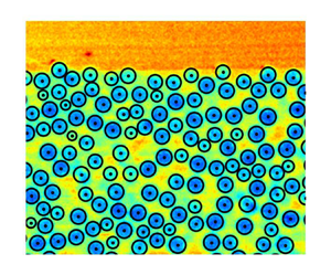
  $90^\circ$ from the enlightened plane. The solid particles appear as black disks in the camera frame. The accurate matching of the refractive index, the thinness of the laser sheet and the resolution of the camera allow the recording of high-quality images with resolution 30 px per particle.
2.3. Measurement methods
2.3.1. Concentration fields
For both suspensions (A and B), the method used to measure the concentration field is the same as in d'Ambrosio et al. (Reference d'Ambrosio, Blanc and Lemaire2021). The concentration field is determined through the measurement of the particle number density  $n_{ij}$ in the
  $(x,z)$ vertical laser plane. To this aim, each image is binarized with a local threshold whose value
  $T(x,z)$ is calculated individually for each pixel
  $(x,z)$ of the image
  $I(x,z)$, where
  $T(x,z)$ is a weighted sum (cross-correlation with a Gaussian window) of a
  $171\,\textrm {px} \times 171\,\textrm {px}$ neighbourhood of the pixel
  $(x,z)$. The particles are detected through a watershed segmentation process (Vincent & Soille Reference Vincent and Soille1991), and the position of the barycentre of each segmented zone gives the position of each particle centre in the
  $(x,z)$ plane sampled with rectangular cells
  $(i,j)$ with edges of sizes
  $\delta x$ and
  $\delta z$. One can note that
  $\delta x$ can be adapted to the purpose of the measurement. For instance, a high resolution allows us to observe particle layering near the walls but is not required to study the outward migration of particles, where the concentration is expected to vary smoothly. For the vertical direction, we have chosen
  $\delta z \sim 2a$ in order to measure
  $\phi (z)$ with a high spatial resolution.
In each cell  $[\delta x\times \delta z]$, the number of particle centres
  $N_{ij}(x,z)$ is measured. The particle density
  $n_{ij}(r,z) = N_{ij}/(\delta x\,\delta y)$ is reconstructed in the
  $(r,z)$ plane, making the change of variable
  $r = \sqrt {y_0^2 + x^2}$. Due to the non-zero thickness of the laser sheet and the slight polydispersity of the particles,
  $n_{ij}$ is not the absolute particle density, and to compute the true particle volume fraction
  $\phi$, we use particle volume conservation:
  $\phi (r,z) = \chi \,n(r,z)$. Depending on the type of suspension (neutrally (A) or negatively (B) buoyant particles), the coefficient
  $\chi$ is determined either from the total height
  $H$ of the suspension imaged by the camera for suspension A, or from the sediment height in the gap,
  $h_0$, and the value of the packing volume fraction of the sediment,
  $\phi _0$, for suspension B:
 \begin{equation} \chi_A = \frac{{\rm \pi} \bar{\varPhi} (R_2^2 - R_1^2) H}{\displaystyle\int_0^H \int_{R_1} ^{R_2} n_{ij} 2{\rm \pi} r\,{\rm d}r\,{\rm d}z} \quad {\rm and} \quad \chi_B = \frac{{\rm \pi}\phi_0 (R_2^2 - R_1^2 ) h_0}{\displaystyle \int_0 ^{h_0} \int_{R_1}^{R_2} n_{ij} 2{\rm \pi} r\,{\rm d}r\,{\rm d}z}, \end{equation}
where  $H$ is the height of suspension A,
  $\bar {\varPhi }$ is the averaged solid volume fraction in suspension A,
  $h_0 = 21.3\,\textrm {mm} \approx 4(R_2 - R_1 )$ is the sediment height in suspension B, and
  $\phi _0 = 0.574 \pm 0.003$ is the packing fraction of the sediment (see d'Ambrosio et al. Reference d'Ambrosio, Blanc and Lemaire2021). Finally,
  $\phi (r,z)$ is averaged over
  $10\,000$ non-correlated images (see figures 2(a) and 4a).

Figure 2. (a) Particle volume fraction maps: examples of solid volume fraction mappings for four different average concentrations of suspension A, namely  $\bar {\varPhi } = 0.414$, 0.458, 0.483 and 0.520. (b) Normalized orthoradial velocity maps: examples of relative velocity mappings
  $v_\theta /\varOmega R_1$ for
  $\varOmega = 1$ rpm for the same
  $\bar {\varPhi }$ as in (a). The inner cylinder (rotor) is located on the left of each map, while the outer cylinder (stator) is on the right. Horizontal resolution is
  $\delta x = 1/14 (R_2-R_1)$.
2.3.2. Velocity fields
The same numerical process is applied to measure the velocity field for both kinds of suspensions. The shift in the laser sheet out of the radial plane allows particle image velocimetry (PIV) measurements (Manneville, Bécu & Colin Reference Manneville, Bécu and Colin2004) in the ( $x,z$) plane. Under the assumption that the radial component of the velocity is much smaller than the azimuthal component,
  $v_\theta$ can be deduced from a simple projection of
  $v_x$ along the orthoradial direction (see figure 1b):
 \begin{equation} v_\theta(x,z) = v_x(x,z)\,\frac{\sqrt{x^2 + y_0^2}}{y_0}. \end{equation}
The velocity field  $\boldsymbol {v}(v_x(x,z),v_z(x,z))$ is computed using the open source software DPIVSOFT (available at https://www.irphe.fr/meunier; Meunier & Leweke Reference Meunier and Leweke2003). Each image is divided into correlation windows of size
  $128\,\textrm {px}\times 128\,\textrm {px}$. Each correlation window contains approximately 10 particles that play the role of PIV tracers. The cross-correlation of the corresponding windows from two successive images yields the mean velocity of the particles in the window. The in-plane loss of pairs error is decreased by translating the correlation windows in a second run (Westerweel Reference Westerweel1997), thus reducing the correlation window size to
  $64\,\textrm {px} \times 64\,\textrm {px}$. The same procedure performed on all windows gives the velocity field, which is averaged over 100 images. The mapping of the
  $\theta$ component of the velocity field in the
  $(x,z)$ plane is then obtained and used to reconstruct the velocity field in the
  $(r,z)$ plane (see figures 2(b) and 4(b)).
3. Concentration and velocity profiles
3.1. Neutrally buoyant suspension A
Steady radial profiles of particle volume fraction were measured for several values of  $\bar {\varPhi } = 0.520, 0.500, 0.483, 0.458, 0.435, 0.414, 0.394$. To measure these profiles, the suspension is first sheared at a constant inner cylinder rotation speed
  $\varOmega =1$ rpm. Throughout the shearing process, the torque to be applied to the inner cylinder to maintain a constant rotation rate is recorded, and when it no longer varies, the migration steady state is considered to have been reached. The typical time and accumulated strain before recording the concentration and velocity fields are of the order of 8 h and 12 000, respectively. Figure 2(a) displays examples of concentration mappings for four different values of
  $\bar {\varPhi }$:
  $0.414$,
  $0.458$,
  $0.483$ and
  $0.52$. One can observe that, as expected, the solid volume fraction
  $\phi$ is vertically homogeneous, while a clear outside migration is visible as well as a decay of
  $\phi$ near the walls. These maps are averaged vertically to obtain the radial
  $\phi$ profiles, shown in figure 3. In agreement with the literature, we observe particle layering that is more and more pronounced as
  $\bar {\varPhi }$ increases (Yeo & Maxey Reference Yeo and Maxey2010; Blanc et al. Reference Blanc, Lemaire, Meunier and Peters2013; Metzger, Rahli & Yin Reference Metzger, Rahli and Yin2013; Gallier et al. Reference Gallier, Lemaire, Lobry and Peters2016; Deboeuf et al. Reference Deboeuf, Lenoir, Hautemayou, Bornert, Blanc and Ovarlez2018; Sarabian et al. Reference Sarabian, Firouznia, Metzger and Hormozi2019). The decay in
  $\phi$ near the walls displayed in figure 2(a) is related to this layering.

Figure 3. Steady radial profiles of the volume fraction  $\phi (r)$ for the different average volume fractions
  $\bar {\varPhi }$. Two main observations can be made in agreement with the literature: (1) the particle layering near the walls, which tends to be larger when
  $\bar {\varPhi }$ increases; (2) the outward migration of the particles, which appears to be even more pronounced when
  $\bar {\varPhi }$ is higher. The inset shows a zoom of the profiles outside the zones where particle layering is observed. Horizontal resolution is
  $\delta x = (R_2- R_1)/200 $.
Once the concentration profile has been measured at  $\varOmega = 1$ rpm, the velocity profiles are measured for several angular speeds of the inner cylinder,
  $\varOmega = 0.1, 0.2, 0.3, 0.5, 0.7,$
  $1, 2$ rpm, in order to study the rheological behaviour of the suspension over a large range of shear stress
  $\varSigma _{12} \in [2,170]\,\textrm {Pa}$. The Reynolds number and the Taylor number are smaller than 1 for all the values of the applied angular velocity (for the highest angular velocity,
  $Re = \rho \varOmega R_1(R_2-R_1)/\eta \sim 10^{-2}$ and
  $Ta = 4\rho ^2\varOmega ^2(R_2-R_1)^4/\eta ^2 \sim 10^{-5}$), and the Péclet number is very large (
 $Pe = 6{\rm \pi} \eta a^3 \dot {\gamma } / k_B T > 10^{10}$). Examples of velocity fields
  $v_\theta (r,z) /\varOmega R_1$ are presented in figure 2(b). As observed for the particle concentration field,
  $v_{\theta }$ does not vary with
  $z$. The
  $z$-averaged radial profiles
  $v_\theta (r)$ are shown in Appendix A (figure 12) for each average concentration
  $\bar {\varPhi }$ and each rotor velocity
  $\varOmega$. The velocity profiles are increasingly deviating from a Newtonian profile as the average concentration
  $\bar {\varPhi }$ increases, in agreement with the literature (Ovarlez et al. Reference Ovarlez, Bertrand and Rodts2006). Besides, it is observed that the wall slip is more and more significant when
  $\bar {\varPhi }$ increases or when
  $\varOmega$ decreases.
3.2. Negatively buoyant suspension B
When the particles are heavier than the suspending liquid, they settle. Under the application of a shear stress, the settled layer expands, resulting in an inhomogeneous vertical concentration profile. We focus on the steady profiles, obtained when the resuspension is completed, for various angular velocities  $\varOmega = 0.3, 0.5, 1, 2, 5, 10, 20, 30, 40, 60$ rpm. The suspension B is first sheared with an angular velocity of the rotor equal to 5 rpm for one hour. Then
  $\varOmega$ is set to the desired value, and the torque applied to the inner cylinder is registered. The acquisition of images begins when the torque becomes constant (after a few hours, which corresponds to a strain of approximately
  $10^4$). For all the experiments, the Reynolds number and the Taylor number are smaller than
  $1$, and the Péclet number is very large (
 $Pe > 10^8$). These procedures are described more thoroughly in d'Ambrosio et al. (Reference d'Ambrosio, Blanc and Lemaire2021), along with the main results that are as follows.
(i) Particle layering is also observed near the walls over a distance of approximately
 $8a\approx (R_2-R_1)/5$ for $\phi \approx 0.55$.
(ii) Outside these zones, the particle volume fraction hardly varies along
$r$ at given $z$, in contrast with what has been observed for the neutrally buoyant suspension.(iii) The concentration decreases slowly with
$z$ in the resuspended layer, and drops sharply to zero at the clear liquid/suspension interface.


These results are illustrated in figure 4.

Figure 4. Volume fraction and orthoradial velocity maps in the resuspension experiments with suspension B for different rotor angular velocity values. (a) Particle volume fraction maps: mapping of the particle volume fraction averaged over 10 000 images (with the exception of  $\varOmega =0$ rpm, for which only 20 images have been averaged). (b) Normalized orthoradial velocity maps: azimuthal velocity normalized by the rotor velocity and averaged over 100 velocity fields. Figure from d'Ambrosio et al. (Reference d'Ambrosio, Blanc and Lemaire2021).
4. Shear viscosity
The purpose of this section is to describe how the relationship between the shear stress and the shear rate is determined for different particle volume fractions through local measurements in the neutrally buoyant suspension (A). It is worth mentioning that the vertical gradient of concentration that is present in the negatively buoyant suspension (B) precludes the determination of the shear stress from the torque applied to the rotor.
4.1. Local viscosity measurement method
The stress field is obtained by solving the Cauchy momentum equation, which for low-Reynolds-number flows (see § 3 for evaluation of the Reynolds number) reduces to
 \begin{equation} \boldsymbol{\nabla}\boldsymbol{\cdot}\boldsymbol{\varSigma} = 0, \end{equation}
which gives
 \begin{equation} \varSigma_{12} = \varSigma_{\theta r} = \frac{C}{r^2}, \quad \textrm{with}\ C = \frac{\varGamma}{2{\rm \pi} H}, \end{equation}
where  $H$ and
  $\varGamma$ are the height of the suspension in the gap and the torque applied on the rotor, respectively. Then from the measurement of the velocity profiles
  $v_{\theta }(r)$, we determine the local relative shear viscosity:
 \begin{equation} \eta_s(r) = \frac{\varSigma_{12}}{\eta_0 \dot{\gamma}}, \end{equation}
with
 \begin{equation} \dot{\gamma}={-}r\,\frac{\partial( v_\theta/r)}{\partial r}. \end{equation}
The viscosity of the suspension is determined outside the layered zones near the walls (see figure 3) since it is well-known that particle layering significantly affects the rheological behaviour (Gallier et al. Reference Gallier, Lemaire, Peters and Lobry2014, Reference Gallier, Lemaire, Lobry and Peters2016) of suspensions. To obtain the variation of the shear viscosity  $\eta _s$ with the shear stress and the particle volume fraction, the shear rate
  $\dot {\gamma }(r)$ is determined for each radial position (using (4.4)) as well as the particle volume fraction
  $\phi (r)$, while the local shear stress
  $\varSigma _{12}(r)$ is given by (4.2). The analysis of all these data shows that, at a given value of
  $\phi$, the suspension behaves as a non-Newtonian shear-thinning fluid (see appendix B).
4.2. Shear-thinning behaviour captured by a stress-dependent jamming volume fraction
Flow curves of shear-thinning suspensions are sometimes fitted by a Herschel–Bulkley law (Coussot & Piau Reference Coussot and Piau1994; Schatzmann, Fischer & Bezzola Reference Schatzmann, Fischer and Bezzola2003; Sosio & Crosta Reference Sosio and Crosta2009; Mueller, Llewellin & Mader Reference Mueller, Llewellin and Mader2010; Vance, Sant & Neithalath Reference Vance, Sant and Neithalath2015). This approach is depicted briefly in Appendix B. However, a more convenient way to capture shear-thinning consists in introducing a stress-dependent jamming volume fraction,  $\phi _m(\varSigma _{12})$ (Wildemuth & Williams Reference Wildemuth and Williams1984; Zhou, Uhlherr & Luo Reference Zhou, Uhlherr and Luo1995; Blanc et al. Reference Blanc, d'Ambrosio, Lobry, Peters and Lemaire2018; Lobry et al. Reference Lobry, Lemaire, Blanc, Gallier and Peters2019). The value of
  $\phi _m$ at a given stress is obtained by measuring the variation of the relative viscosity with the volume fraction, which, as displayed in figure 5, can be adjusted by a Maron–Pierce law:
 \begin{equation} \eta_r(\varSigma_{12})= \left( 1 - \frac{\phi}{\phi_m(\varSigma_{12})} \right)^{{-}2}. \end{equation}
Figure 5. Relative viscosity  $\eta _s$ as function of
  $\phi /\phi _m(\varSigma _{12})$. Each symbol corresponds to the local measurement of the viscosity and of the particle volume fraction
  $\phi _m$ being deduced from the local shear stress value (4.6). Each colour labels
  $\bar {\varPhi }$ values 0.520 (blue), 0.500 (black), 0.483 (red), 0.458 (orange), 0.435 (purple), 0.414 (brown), 0.394 (green). The black dashed line corresponds to the Maron–Pierce law:
  $\eta _s = (1-\phi /\phi _m)^{-2}$.
More precisely, we obtained the variation of  $\phi _m$ with
  $\varSigma _{12}$ by fitting the variation of
  $1/\sqrt {\eta _r}$ with
  $\phi$ at a given shear stress. Figure 15 in Appendix C shows these fittings for different values of the local shear stress. It is worth noting that the Maron–Pierce law, although globally adequate to represent the variation of the viscosity with the volume fraction, is not respected perfectly for the largest volume fractions for which the exponent tends to decrease. A better fit could have been obtained by introducing, as is often done (Blanc et al. Reference Blanc, d'Ambrosio, Lobry, Peters and Lemaire2018; Singh et al. Reference Singh, Mari, Denn and Morris2018; Lobry et al. Reference Lobry, Lemaire, Blanc, Gallier and Peters2019), a second free parameter in the Maron–Pierce law:
  $\eta _r(\varSigma _{12})= \alpha (\varSigma _{12})(1 - {\phi }/{\phi _m(\varSigma _{12})})^{-2}$. However, we have chosen to limit the number of free parameters in the constitutive law in order to facilitate the analysis of the data that will be presented below, in particular in §§ 6 and 7. Furthermore, figure 5 shows that with this one-parameter fitting, the experimental data approximately line up on a single curve, which provides a consistency check for the fitting procedure.
The variation of  $\phi _m$ with
  $\varSigma _{12}$ is displayed in figure 6, where it is observed that
  $\phi _m$ increases from 0.54 to 0.59 when the shear stress increases from
  $5$ to 90 Pa, illustrating the shear-thinning behaviour of the suspension. Besides, one can note that the values of
  $\phi _m$ are in the typical range reported in the literature for frictional non-Brownian suspensions (Zarraga et al. Reference Zarraga, Hill and Leighton2000; Ovarlez et al. Reference Ovarlez, Bertrand and Rodts2006; Boyer et al. Reference Boyer, Guazzelli and Pouliquen2011; Peters et al. Reference Peters, Ghigliotti, Gallier, Blanc, Lemaire and Lobry2016; Singh et al. Reference Singh, Mari, Denn and Morris2018; Blanc et al. Reference Blanc, d'Ambrosio, Lobry, Peters and Lemaire2018; Lobry et al. Reference Lobry, Lemaire, Blanc, Gallier and Peters2019; Arshad et al. Reference Arshad, Maali, Claudet, Lobry, Peters and Lemaire2021). In figure 6, we have also plotted a power-law fitting curve (black line) that will be used in the following when we need to estimate the local value of the jamming fraction, knowing the local value of the stress:
 \begin{equation} \phi_m=0.515\varSigma_{12}^{0.0286}. \end{equation}
Figure 6. Jamming volume fraction  $\phi _m$ as a function of the shear stress
  $\varSigma _{12}$ deduced from figure 15. Black line: power-law fit,
  $\phi _m =0.515\varSigma _{12}^{0.0286}$. Grey: confidence interval.
This power law is valid only on the shear stress domain that has been investigated, and has no physical meaning. It would have been possible to fit our data by a law of the type of Lobry et al. (Reference Lobry, Lemaire, Blanc, Gallier and Peters2019), which corresponds to a variation of  $\phi _m$ with stress driven by a decrease in the pairwise friction coefficient when
  $\varSigma _{12}$ increases. Indeed, the range of variation of
  $\phi _m$ with
  $\varSigma _{12}$ is fully consistent with what is predicted for shear-thinning induced by a variable friction coefficient between particles. But for the sake of simplicity in data analysis, we chose the simple power law of (4.6).
5. The characterization of $\varSigma _{22}^p$

Figure 3 displays the radial  $\phi$ profiles measured for different values of the averaged volume fraction of suspension A. Outside the near wall regions, the particle volume fraction increases approximately linearly with
  $r$. In this section, we will make use of this outward particle migration to deduce
  $\varSigma _{22}^p$.
5.1. Theoretical approach
According to the SBM (Morris & Boulay Reference Morris and Boulay1999), in the absence of inertial effects, the steady particle concentration profile satisfies the balance of particle normal stresses:
 \begin{equation} \boldsymbol{\nabla}\boldsymbol{\cdot}\boldsymbol{\varSigma}^p = 0. \end{equation}
In the present study, as mentioned earlier, the flow Reynolds number is small. Nevertheless, rigorously speaking, (5.1) is valid only for the case of zero inertia. In the presence of inertial effects, obtaining a conservation equation for the particle phase is not trivial. However, Badia et al. (Reference Badia, D'Angelo, Peters and Lobry2022) showed recently that in the case where the relative velocity of the two phases may be neglected compared to the average velocity in all inertial terms, inertia can be accounted for by writing the equation
 \begin{equation} \boldsymbol{\nabla}\boldsymbol{\cdot}\boldsymbol{\varSigma}^p ={-}\phi (\rho_p-\rho_f)\left[\boldsymbol{g}-\frac{{\rm D}\boldsymbol{v}}{{\rm D}t}\right]. \end{equation}
 Thus the inertial term is proportional to  $(\rho _p-\rho _f)$ and can be neglected in such a way that (5.1) can be used.
Then in the velocity gradient direction, we obtain
 \begin{equation} \frac{1}{r}\,\frac{\partial (r\varSigma_{22}^p)}{\partial r} - \frac{\varSigma_{11}^p}{r} = 0, \end{equation}
which can be written as
 \begin{equation} \frac{\partial \varSigma_{22}^p}{\partial r} - \frac{N_1^p}{r} = 0, \end{equation}
where  $N_1^p$ is the first particle normal stress difference:
  $N_1^p = \varSigma _{11}^p - \varSigma _{22}^p$.
Following Morris & Boulay (Reference Morris and Boulay1999),  $\varSigma _{22}^p$ can be rewritten as
  $\varSigma _{22}^p = -\lambda _2\eta _0\eta _n\dot {\gamma }$, with
  $\lambda _2 = \varSigma _{22}^p / \varSigma _{11}^p$ and
  $N_1^p=-\eta _0 \eta _n\dot {\gamma }(1-\lambda _2)$, which gives
 \begin{equation} q_2(\phi, \phi_m) \equiv \frac{\eta_n(\phi,\phi_m)}{\eta_s(\phi, \phi_m)} ={-}\frac{\varSigma_{22}^p}{\varSigma_{12}}. \end{equation}
According to (4.2), this equation can be rewritten as
 \begin{equation} q_2(r) =\left(\frac{q_2(r_0)}{r_0^{(1+\lambda_2)/\lambda_2}}\right) \times r^{(1+\lambda_2)/\lambda_2}=Q_2(\varPhi_0) \times r^{(1+\lambda_2)/\lambda_2}, \end{equation}
where  $r_0$ is any radial position in the gap at which the particle volume fraction is equal to
  $\varPhi _0$.
The exact value of  $\lambda _2$ is still debated. Nevertheless, several numerical studies (Gallier et al. Reference Gallier, Lemaire, Peters and Lobry2014; Lobry et al. Reference Lobry, Lemaire, Blanc, Gallier and Peters2019) showed that
  $N_1^p \ll \varSigma _{12}$. In the case of frictional particles (
 $\mu \approx 0.5$), Gallier et al. (Reference Gallier, Lemaire, Peters and Lobry2014) showed
  $N_1^p / \varSigma _{12} \lesssim 10^{-2}$, while
  $\varSigma _{22}^p$ is of the same order as
  $\varSigma _{12}$ (Zarraga et al. Reference Zarraga, Hill and Leighton2000; Dbouk et al. Reference Dbouk, Lobry and Lemaire2013; Gallier et al. Reference Gallier, Lemaire, Peters and Lobry2014), leading to
  $\lambda _2\approx 1$. In the following, we will pursue the analysis with three values of
  $\lambda _2$, namely
  $0.8$,
  $1$ and
  $1.2$, and we will show that the values of
  $q_2$ hardly vary with
  $\lambda _2$ (values between
  $0.8$ and
  $1.2$).
5.2. Determination of $q_2 = -\varSigma _{22}^p/\varSigma _{12}$

In this subsection, we want to establish the variation of  $q_2 = -\varSigma _{22}^p/\varSigma _{12}$ as a function of the ratio
  $\phi /\phi _m$. We compute
  $\phi _m(r)$ from
  $\varSigma _{12}(r)$ and (4.6) so that
  $\phi /\phi _m$ is known for each radial position. However, it is essential to understand that, so far, we do not know the value
  $Q_2$ in (5.6), and the main issue is to find a way to determine it.
In order to obtain the value of  $Q_2$, at a given position
  $r_0$ and for a given ratio
  $\phi (r_0)/\phi _m(r_0)$, we use the correlation proposed by Zarraga et al. (Reference Zarraga, Hill and Leighton2000):
 \begin{equation} q_2(\phi/\phi_m)={-}2.17\times0.62^3 (\phi/\phi_m)^3\exp({2.34\times 0.62 (\phi/\phi_m)}), \end{equation}
where 0.62 is the jamming volume fraction obtained by Zarraga et al. (Reference Zarraga, Hill and Leighton2000) for  $\dot {\gamma }=10\,\textrm {s}^{-1}$. Although the suspensions studied by these authors present a noticeable shear-thinning behaviour, Zarraga et al. (Reference Zarraga, Hill and Leighton2000) did not address how to introduce the shear-thinning behaviour into the constitutive laws that relate particle normal stresses to shear stress. We consider here that a possibility would be to write the constitutive laws as a function of
  $\phi /\phi _m$ – rather than as a function of
  $\phi$ – because, since the shear viscosity has been shown to be a function of the sole ratio
  $\phi /\phi _m$ (see § 4), writing the same for the particle normal stresses is the only way to keep a linear relation between
  $\varSigma _{22}^p$ and
  $\varSigma _{12}$.
To set  $Q_2$, we chose
  $r_0 \approx R_1 + 0.66\times (R_2-R_1)$, where the ratio
  $\phi /\phi _m$ is the largest outside the layered regions (see the blue curve in figure 3 obtained for
  $\bar {\varPhi }=0.52$). At this position,
  $\phi /\phi _m = 0.93$ and (5.7) gives
  $Q_2 = 1.604$. This chosen reference point corresponds to the most extreme right point in figure 7. Now that the reference is set, (5.6) straightforwardly provides
  $q_2(\phi /\phi _m)$ for all the values of
  $\phi /\phi _m$ obtained from the migration profile measured at
  $\bar {\varPhi } = 0.52$ (the blue circles in figure 7). Next, we deal with the averaged concentration immediately smaller than
  $0.52$, i.e.
  $\bar {\varPhi }=0.50$. For this new average concentration, the value of
  $Q_2$ is determined using the value of
  $q_{2}$ obtained with
  $\bar {\varPhi }=0.52$ over the overlap range of
  $\phi /\phi _m$. This enables us to plot the black circles in figure 7. We proceed in this same way for all the migration profiles measured at decreasing values of
  $\bar {\varPhi }$ in order to build piece by piece the whole curve of figure 7. The coloured circles have been obtained by setting
  $\lambda _2=1$, while the two grey lines that delimit the grey zone correspond to the determination of
  $q_2$ with
  $\lambda =0.8$ (lower curve) and
  $\lambda =1.2$ (upper curve). Thus the choice of the exact value of
  $\lambda _2$ is not critical and affects the
  $q_2$ values.

Figure 7. Variation of the function  $q_2 = \eta _n / \eta _s = \varSigma _{22}^p / \varSigma _{12}$ with the ratio
  $\phi /\phi _m$. The colour code is the same as in figure 15, for average concentration
  $\bar {\varPhi }$ values 0.520 (blue), 0.500 (black), 0.483 (red), 0.458 (orange), 0.435 (purple), 0.414 (brown), and 0.394 (green). Green solid line: correlation of Zarraga et al. (Reference Zarraga, Hill and Leighton2000) (
 $\phi _m = 0.62$). The two grey lines that delimit the grey zone correspond to the determination of
  $q_2$ with
  $\lambda =0.8$ (lower curve) and
  $\lambda =1.2$ (upper curve). Black solid line: correlation of Boyer et al. (Reference Boyer, Guazzelli and Pouliquen2011) (
 $\phi _m = 0.585$). Red dashed line: polynomial fit
  $q_2 = 5.47(\phi /\phi _m)^2-3.35(\phi /\phi _m)$.
We would also like to point out that all the results presented in figure 7 rely on the choice of the first value of  $Q_2$ that we have used. Another choice of the value of
  $Q_2$ would have resulted in a curve with the same shape but shifted vertically. However, we are quite confident in our choice since the two most used correlations in the literature, those of Zarraga et al. (Reference Zarraga, Hill and Leighton2000) (green line in figure 7) and Boyer et al. (Reference Boyer, Guazzelli and Pouliquen2011) (black line in figure 7), give almost the same value of
  $q_2$ for the value of
  $\phi /\phi _m$ chosen to set the reference.
In figure 7, the correlation proposed by Zarraga et al. (Reference Zarraga, Hill and Leighton2000) (with  $\phi _m=0.62$) is also plotted, and rather good agreement with our results is observed even though there is a slight mismatch for the lowest values of
  $\phi /\phi _m$. On the contrary, the consistency between our results and the correlation proposed by Boyer et al. (Reference Boyer, Guazzelli and Pouliquen2011) is less satisfactory, but we have to keep in mind that the work of Boyer et al. (Reference Boyer, Guazzelli and Pouliquen2011) focuses mainly on very dense suspensions, as will be discussed in § 7.
6. The characterization of $\varSigma _{33}^p$

Here, we study the rheological behaviour of the negatively buoyant suspension B in order to determine the third particle normal stress  $\varSigma _{33}^p$. This section may be considered as a next step of our previous work on viscous resuspension (d'Ambrosio et al. Reference d'Ambrosio, Blanc and Lemaire2021), where we determined
  $\varSigma _{33}^p$ from the local measurements of
  $\phi (z)$ by solving the particle stress balance in the vertical direction. We start from the
  $z$ projection of the total stress balance:
 \begin{equation} \frac{1}{r}\,\frac{\partial\left(r\varSigma_{23}\right)}{\partial r} + \frac{\partial \varSigma_{33}}{\partial z}=\Delta \rho\,g \phi. \end{equation}
We first showed, thanks to the analysis of the velocity profiles measured in the resuspension experiments, that the first left-hand-side term can be neglected, leading to the following simple equation for the third particle normal stress (see supplementary material of d'Ambrosio et al. Reference d'Ambrosio, Blanc and Lemaire2021):
 \begin{equation} \frac{\partial \varSigma_{33}^p}{\partial z} = \Delta\rho\,g \phi, \end{equation}
with the boundary condition  $\varSigma _{33}^p=0$ for
  $z=h$, where
  $h$ denotes the height of the interface between the resuspended layer and the clear fluid. Besides, we derived the local shear rate
  $\dot {\gamma }(r,z)$ from the measurement of the azimuthal velocity field
  $v_\theta (r,z)$. In agreement with the work of Saint-Michel et al. (Reference Saint-Michel, Manneville, Meeker, Ovarlez and Bodiguel2019), we highlighted the nonlinear variation of
  $\varSigma _{33}^p$ with
  $\dot {\gamma }$:
 \begin{equation} \frac{\varSigma_{33}^p}{\eta_0\dot{\gamma}^{n}} = f(\phi), \quad \textrm{with}\ n=0.7. \end{equation}
This nonlinear behaviour raises questions. On the one hand, it is anticipated that  $\varSigma _{33}^p$ does not vary linearly with
  $\dot {\gamma }$ since it is expected to be proportional to the shear stress, which itself may not vary linearly with shear rate (see, for instance, Tanner (Reference Tanner2018) or Zarraga et al. (Reference Zarraga, Hill and Leighton2000) and Appendix B). But on the other hand, the exponent in the shear stress versus shear rate relation is all but constant and decreases when the particle fraction increases (see Appendix B), which disagrees with (6.3). In this section, we will show that the relation between
  $\varSigma _{33}^p$ and
  $\varSigma _{12}$ is linear, and that
  $\varSigma _{33}^p/(\eta _0\dot {\gamma })$ is a function of only
  $\phi /\phi _m$.
6.1. Determination of the shear stress field in viscous resuspension experiments
As mentioned earlier, the shear stress cannot be deduced from the torque applied to the rotor since the particle volume fraction varies along the  $z$ direction, which precludes the assumption that the stress is vertically homogeneous. To determine
  $\varSigma _{12}(r,z)$, we make the hypothesis that suspensions A and B obey the same constitutive laws (see § 4.2):
 \begin{equation} \eta_s(\phi,\phi_m) = (1 - \phi/\phi_m)^{{-}2} \quad \textrm{and} \quad \phi_m =0.515\varSigma_{12}^{0.0286}. \end{equation}
 Thus from the local measurement of  $\phi (r,z)$ and
  $\dot {\gamma }(r,z)$, the local shear stress
  $\varSigma _{12}(r,z)$ can be deduced from (6.4a,b) and the implicit equation
 \begin{equation} \varSigma_{12}(r,z) = \eta_s(\phi(r,z), \phi_m(\varSigma_{12})) \times \dot{\gamma}(r,z). \end{equation}
 Using this equation is possible because, as shown in the supplementary material of d'Ambrosio et al. (Reference d'Ambrosio, Blanc and Lemaire2021), the  $13$-component of the rate of deformation tensor is very small compared to the
  $12$-component. The local jamming volume fraction
  $\phi _m(r,z)$ is then determined from
  $\varSigma _{12}(r,z)$.
Note that assuming that suspensions A and B obey the same constitutive law (6.4a,b) is a rather strong hypothesis that is difficult to justify a priori. However, the facts that the particles are exactly the same for both suspensions and that the suspending fluids are quite similar (both based on water/Triton X-100 mixtures) make this hypothesis quite reasonable. Moreover, we will see in the next two subsections that the use of this assumption provides consistent results, in agreement with the literature with, in particular, the linear variation of  $\varSigma _{33}^p$ with
  $\varSigma _{12}$ and the measurement of the ratio
  $\varSigma _{33}^p/\varSigma _{22}^p\approx 0.5$.
6.2. Variation of $\varSigma _{33}^p$ with $\varSigma _{12}$


Figure 8 displays the variation of the third particle normal stress  $-\varSigma _{33}^p$ with the shear stress
  $\varSigma _{12}$ for different values of
  $\phi /\phi _m$, targeted across all the different experiments of viscous resuspension done with suspension B. Although the data dispersion is rather large, we observe that a linear relation exists between
  $\varSigma _{33}^p$ and
  $\varSigma _{12}$, in agreement with the literature (Guazzelli & Pouliquen Reference Guazzelli and Pouliquen2018).

Figure 8. Variation of the third particle normal stress  $-\varSigma _{33}^p$ with the shear stress
  $\varSigma _{12}$ for different values of
  $\phi /\phi _m$. Black lines: linear fits. Each symbol colour corresponds to a resuspension experiment performed with a given angular velocity of the rotor,
  $\varOmega$: 0.3 rpm (blue), 0.5 rpm (orange), 1 rpm (green), 2 rpm (red), 5 rpm (purple), 10 rpm (brown), 20 rpm (pink), 30 rpm (gray), 40 rpm (olive), 60 rpm (cyan).
6.3. Shear-thinning behaviour of $\varSigma _{33}^p$

In figure 9(a), we have reproduced the variation of  $-\varSigma _{33}^p/\eta _0\dot {\gamma }$ with
  $\phi$, already displayed in our previous paper (d'Ambrosio et al. Reference d'Ambrosio, Blanc and Lemaire2021). The colour scale indicates the value of
  $\varSigma _{12}$ for each point, deduced from (6.4a,b) and (6.5). We observe that for a given value of
  $-\varSigma _{33}^p/\eta _0\dot {\gamma }$, the shear stress tends to increase as
  $\phi$ rises. This observation suggests that the thickness of the curve is not due to experimental noise but rather, the particle volume fraction is not the only variable controlling the value of the ratio
  $-\varSigma _{33}^p/\eta _0\dot {\gamma }$. The dispersion of the data is reduced significantly when this ratio is plotted against
  $\phi /\phi _m$, where
  $\phi _m$ is a function of the shear stress, as shown in figure 9(b). This observation is consistent with the linear variation of
  $\varSigma _{33}^p$ with
  $\varSigma _{12}$ presented in the previous subsection together with the shear-thinning behaviour of the suspension, and provides a plausible physical explanation for the nonlinear behaviour of
  $\varSigma _{33}^p$ with
  $\dot {\gamma }$ recorded by both Saint-Michel et al. (Reference Saint-Michel, Manneville, Meeker, Ovarlez and Bodiguel2019) and d'Ambrosio et al. (Reference d'Ambrosio, Blanc and Lemaire2021), as discussed in the introduction of § 6.

Figure 9. Variation of the ratio  $-\varSigma _{33}^p/\eta _0\dot {\gamma }$ as a function of (a)
  $\phi$ and (b) of
  $\phi /\phi _m$. The colour bars display the values of the shear stress calculated from (6.4a,b) and (6.5). The correlation of Zarraga et al. (Reference Zarraga, Hill and Leighton2000) with
  $\phi _m =0.62$ is also plotted (green line) as well as the results of Boyer et al. (Reference Boyer, Guazzelli and Pouliquen2011) with
  $\phi _m=0.585$, considering
  $\varSigma _{33}^p/\varSigma _{22}^p=0.5$ (black line). The solid lines show the domains where these laws have been determined experimentally, while the dashed lines correspond to extrapolations of the data.
In figure 9(b), the correlations proposed by Boyer et al. (Reference Boyer, Guazzelli and Pouliquen2011) (black solid line) and Zarraga et al. (Reference Zarraga, Hill and Leighton2000) (green solid line) are also plotted. It is observed that our results are in good agreement with each of these two correlations in the domains of  $\phi /\phi _m$ in which they have been originally determined:
  $\phi /\phi _m\in [0.48, 0.89]$ for Zarraga et al. (Reference Zarraga, Hill and Leighton2000), and
  $\phi /\phi _m\in [0.7, 0.999]$ for Boyer et al. (Reference Boyer, Guazzelli and Pouliquen2011). But neither the law proposed by Boyer et al. (Reference Boyer, Guazzelli and Pouliquen2011) nor the one proposed by Zarraga et al. (Reference Zarraga, Hill and Leighton2000) is valid on the whole range of values of
  $\phi /\phi _m$ explored in the present study. This point will be discussed again in § 7.
To conclude, the shear rate dependence of  $\varSigma _{33}^p$ can be captured by the variation of the jamming fraction with the shear stress, as is done frequently for the shear viscosity. We have shown that
  $\varSigma _{33}^p$ is proportional to
  $\varSigma _{12}$, which provides a satisfactory physical explanation for the nonlinear variation of
  $\varSigma _{33}^p$ with
  $\dot {\gamma }$ observed by Saint-Michel et al. (Reference Saint-Michel, Manneville, Meeker, Ovarlez and Bodiguel2019) and d'Ambrosio et al. (Reference d'Ambrosio, Blanc and Lemaire2021).
7. $\mu (J)$ rheology

Our results obtained with both suspensions A and B can be used to write the constitutive laws  $\mu =\varSigma _{12}/\varSigma _{22}^p$ and
  $\phi /\phi _m$ as a function of
  $J=\eta _0\dot {\gamma }/\varSigma _{22}^p$, in the frame of the
  $\mu (J)$ rheology proposed by Boyer et al. (Reference Boyer, Guazzelli and Pouliquen2011). It is straightforward to deduce these constitutive laws from the determination of
  $\varSigma _{22}^p$ obtained from the measurement of the radial profile of particle volume fraction carried on the neutrally buoyant suspension, together with the measurement of the local shear rate.
In addition, the viscous resuspension experiments carried out on suspension B can be used. In figure 10, the ratio  $\lambda _{32}=\varSigma _{33}^p/\varSigma _{22}^p=\varSigma _{33}^p/q_2\varSigma _{12}$ is plotted as a function of
  $\phi /\phi _m$ in the range where
  $q_2$ has been measured (
 $\phi /\phi _m\in [0.7,0.95]$; see figure 7). The quite wide scattering of the data is likely related to the limited accuracy of the measurement of
  $\varSigma _{33}^p$ as a function of the ratio
  $\phi /\phi _m$, already observed in figure 9(b). It should also be noted that in these two figures, all of the data points are reported without any averaging, which also contributes to the scattering. Despite the data dispersion, the good thing is that the typical value measured for the ratio
  $\lambda _{32}$ is close to the values found in the literature. In the original SBM (Morris & Boulay Reference Morris and Boulay1999), this ratio is approximated by a constant that is independent of the particle volume fraction and approximately equal to
  $0.6$ (the ratio of
  $\lambda _3\approx 0.5$ over
  $\lambda _2\approx 0.8$ in the SBM). Note that in the present study, we have set
  $\lambda _2=1$, which would lead to
  $\lambda _{32}\approx 0.5$. Even though the scatter of the data in figure 10 is rather large, it is quite satisfactory that
  $\lambda _{32}$ hardly varies with
  $\phi /\phi _m$, that the slight decrease is very similar to what has been measured by Dbouk et al. (Reference Dbouk, Lobry and Lemaire2013) and that the average measured value is
  $0.456$, in rather good agreement with what was expected. It has also to be noted that this value is very close to the result reported by Zarraga et al. (Reference Zarraga, Hill and Leighton2000), who have found
  $\varSigma _{33}^p/\varSigma _{22}^p=0.46$.

Figure 10. Variation of the coefficient  $\lambda _{32} = \varSigma _{33}^p/\varSigma _{22}^p = \lambda _3/\lambda _2$ against the ratio
  $\phi /\phi _m$. The red line shows the Dbouk et al. (Reference Dbouk, Lobry and Lemaire2013) result:
  $\lambda _{32} = (-0.0153 \phi _m \times \phi /\phi _m +0.547 ) / (1.4\phi _m \times \phi /\phi _m + 0.665)$, with
  $\phi _m = 0.58$. The black dashed line indicates the averaged value of
  $\lambda _{32}=0.456$. Each symbol colour corresponds to a resuspension experiment at a given angular velocity of the rotor, i.e.
  $\varOmega$ values 0.3 rpm (blue), 0.5 rpm (orange), 1 rpm (green), 2 rpm (red), 5 rpm (purple), 10 rpm (brown), 20 rpm (pink), 30 rpm (gray), 40 rpm (olive).
In the following, we will use  $\lambda _{32}=0.456$ to deduce
  $J$ and
  $\mu$ from the resuspension experiments:
 \begin{equation} \mu = \lambda_{32} \times \varSigma_{12}/\varSigma_{33}^p \quad {\rm and} \quad J = \lambda_{32} \times \eta_0\dot{\gamma}/\varSigma_{33}^p. \end{equation}
 The variations of  $(1-\phi /\phi _m)$ and
  $\mu$ with
  $J$ are plotted in figures 11(a) and 11(b), respectively. The thick black line corresponds to the results obtained from the measurement of the radial profile in the neutrally buoyant suspension, while the coloured circles have been deduced from the resuspension experiments. First, note that figure 11(a) does not provide any new information since it is strictly equivalent to what was plotted in figure 9(b). Second, it should be mentioned that the uncertainty on the measurements obtained for
  $J\lesssim 10^{-3}-10^{-2}$ is quite large since the uncertainty on both
  $\phi$ and
  $\phi _m$ is of the order of 1 %, which leads to an absolute error on
  $(1-\phi /\phi _m)$ of the order of
  $10^{-2}$. Nevertheless, the present results are rather consistent with the results of Boyer et al. (Reference Boyer, Guazzelli and Pouliquen2011), Tapia et al. (Reference Tapia, Pouliquen and Guazzelli2019) and Etcheverry (Reference Etcheverry2022) (respectively, the green, purple and dark teal curves in figures 11(a) and 11(b)), who observed a variation of
  $(1-\phi /\phi _m)$ in
  $J^{1/2}$ for
  $J<10^{-1}$. For higher values of
  $J$, the variation of
  $(1-\phi /\phi _m)$ with
  $J$ deviates from the above scaling, and our results show very good agreement with those of Zarraga et al. (Reference Zarraga, Hill and Leighton2000) (yellow solid curve). Note that this observation is completely equivalent to the one that we made when discussing the graph in figure 9(b).

Figure 11. (a) Variation of  $(1 - \phi /\phi _m)$ with
  $J$. (b) Variation of
  $\mu$ with
  $J$. The thick black line corresponds to the results extracted from the radial migration profiles (suspension A). The coloured circles correspond to the results obtained through the study of the viscous resuspension (suspension B) for various angular velocities (same colour code as in figure 10). The yellow, green, purple and dark teal lines correspond to the results obtained by Zarraga et al. (Reference Zarraga, Hill and Leighton2000), Boyer et al. (Reference Boyer, Guazzelli and Pouliquen2011), Tapia et al. (Reference Tapia, Pouliquen and Guazzelli2019) and Etcheverry (Reference Etcheverry2022), respectively. Our data show clear agreement with the results of Boyer et al. (Reference Boyer, Guazzelli and Pouliquen2011) for
  $J<{O}(10^{-1})$, and with those of Zarraga et al. (Reference Zarraga, Hill and Leighton2000) for
  $J>{O}(10^{-1})$. The rheological behaviour over the whole range of investigated viscous numbers is captured by introducing a smooth transition function that interpolates between the law proposed by Boyer et al. (Reference Boyer, Guazzelli and Pouliquen2011) and that obtained by Zarraga et al. (Reference Zarraga, Hill and Leighton2000) (see (7.2) and (7.7)). The value
  $J_c=6\times 10^{-2}$ is given by the best fit of (7.2) to the experimental variation of
  $(1-\phi /\phi _m)$ with
  $J$ (red dashed line in (a)). The fitting of Boyer's correlation to the variation of
  $\mu$ with
  $J$ deduced from the radial migration profiles (suspension A) for
  $J\in [3\times 10^{-3}, J_c]$ yields
  $\mu _c=0.39$ and
  $A_\mu =3.7$. The best fit is shown in the inset of (b). The red dashed line in (b) is the result of (7.7) with
  $J_c=6\times 10^{-2}$,
  $A_\mu =3.7$ and
  $\mu _c=0.39$.
Hence the variation of  $1-\phi /\phi _m$ as a function of
  $J$ that has been obtained from the measurements of the vertical concentration profiles in the resuspension experiments seems to be able to bridge the gap between the scalings proposed by Boyer et al. (Reference Boyer, Guazzelli and Pouliquen2011) for
  $J\lesssim 10^{-1}$ on the one hand, and by Zarraga et al. (Reference Zarraga, Hill and Leighton2000) for
  $J\gtrsim 10^{-1}$ on the other hand. Our results on the whole range of investigated viscous numbers (
 $10^{-4}< J<30$) are well fitted by introducing a smooth transition function
  $\mathcal {T}(J/J_c)$ that interpolates between the law proposed by Boyer et al. (Reference Boyer, Guazzelli and Pouliquen2011) (
 $\mathcal {B}_\phi (J)$ hereafter), and that obtained by Zarraga et al. (Reference Zarraga, Hill and Leighton2000) (
 $\mathcal {Z}_\phi (J)$ hereafter):
 \begin{equation} 1-\frac{\phi}{\phi_m}=\mathcal{T}\left(\frac{J}{J_c}\right) \mathcal{B}_\phi(J)+\left(1-\mathcal{T}\left(\frac{J}{J_c}\right)\right)\mathcal{Z}_\phi(J), \end{equation}
where
 \begin{gather} \mathcal{T}(x) = \frac{1}{2}\left(1+\frac{1-x^2}{1+x^2}\right), \end{gather}
 \begin{gather}\mathcal{B}_\phi(J) = 1-\frac{1}{1+J^{1/2}}, \end{gather}
 \begin{gather}\mathcal{Z}_\phi(J) = \frac{J^{1/3}}{A_z+J^{1/3}}, \quad \mathrm{with}\ A_z \approx 1.25, \end{gather}
where  $\mathcal {Z}_\phi$ is deduced from the correlations proposed by Zarraga et al. (Reference Zarraga, Hill and Leighton2000) to relate
  $\varSigma _{22}^p$ to
  $\varSigma _{12}$, and
  $\eta _s$ to
  $\phi$, together with the definition of the viscous number
  $J=\eta _0\dot {\gamma }/\varSigma _{22}^p=(1/\eta _s)(\varSigma _{12}/\varSigma _{22}^p)$.
The red dashed line in figure 11(a) shows the result of the best fit, which yields  $J_c=6\times 10^{-2}$, a value close to the quite abrupt change of slope observed in figure 11(a).
Our data on the variation of  $\mu$ with
  $J$ are plotted in figure 11(b) together with the results of Zarraga et al. (Reference Zarraga, Hill and Leighton2000) in the range
  $J\in [3\times 10^{-3},2]$ (yellow solid line) and the results of Boyer et al. (Reference Boyer, Guazzelli and Pouliquen2011) (green line), Tapia et al. (Reference Tapia, Pouliquen and Guazzelli2019) (purple line) and Etcheverry (Reference Etcheverry2022) (dark teal line) obtained with
  $J<10^{-1}$. Our results are consistent with those of Zarraga et al. (Reference Zarraga, Hill and Leighton2000) and in a rather good agreement with those of Boyer et al. (Reference Boyer, Guazzelli and Pouliquen2011) and Tapia et al. (Reference Tapia, Pouliquen and Guazzelli2019) for small values of
  $J$, even though we measured slightly higher effective friction coefficients for the smallest
  $J$ values. Before going further, it is necessary to recall that the measurements at small
  $J$ values suffer from a large uncertainty: the uncertainty evaluated on the ratio
  $\phi /\phi _m$ is
  ${O}(10^{-2}$), which results in a relative uncertainty of more than
  $50\,\%$ on the evaluation of the shear stress for
  $(1-\phi /\phi _m)\approx 0.04$, i.e.
  $J\approx 10^{-3}$. To this, must be added the uncertainty on
  $\varSigma _{33}^p$ that is likely to be of the same order of magnitude. The uncertainty on the values of
  $\mu$ determined from the radial migration profiles measured in suspension A is much smaller. That is why we decided to determine the law
  $\mu (J)$ on the basis of these last results obtained for
  $J> 3\times 10^{-3}$.
We fit our results obtained with suspension A (black thick curve in figure 11b) in the range  $J\in [3\times 10^{-3},J_c]$ to the correlation proposed by Boyer et al. (Reference Boyer, Guazzelli and Pouliquen2011) in the limit of small
  $J$ (DeGiuli et al. Reference DeGiuli, Düring, Lerner and Wyart2015; Trulsson, DeGiuli & Wyart Reference Trulsson, DeGiuli and Wyart2017; Tapia et al. Reference Tapia, Pouliquen and Guazzelli2019) in order to reduce the number of free parameters:
 \begin{equation} \mathcal{B}_\mu(J) =\mu_c+A_\mu J^{1/2}. \end{equation}
The best fit of our data yields  $A_\mu =3.7$ and
  $\mu _c=0.39$. This value of
  $\mu _c$ is slightly higher but not significantly different from the values given by Boyer et al. (Reference Boyer, Guazzelli and Pouliquen2011) and Tapia et al. (Reference Tapia, Pouliquen and Guazzelli2019), i.e.
  $\mu _c=0.32$ and
  $0.37$, respectively. Furthermore, the inset of figure 11(b) shows that taking
  $\mu _c=0.39$ enables us to obtain the expected behaviour,
  $\mu -\mu _c\propto J^{1/2}$, as well for the neutrally buoyant suspension (black line) as for the non-neutrally buoyant one (circles) for
  $J\lesssim 10^{-1}$. The value of
  $A_\mu$ is between the value measured by Boyer et al. (Reference Boyer, Guazzelli and Pouliquen2011),
  $1.46$, and the value measured by Tapia et al. (Reference Tapia, Pouliquen and Guazzelli2019),
  $5.45$ and comparable to the values reported by Dagois-Bohy et al. (Reference Dagois-Bohy, Hormozi, Guazzelli and Pouliquen2015),
  $A_\mu =4.0$, and recently by Etcheverry (Reference Etcheverry2022),
  $A_\mu =3.05$.
Finally, the variation  $\mu (J)$ measured over the whole range of viscous numbers can again be represented by using the same smooth transition function
  $\mathcal {T}(J/J_c)$ that was employed previously to capture the variation of
  $1-\phi /\phi _m$ with
  $J$ (see (7.3)):
 \begin{equation} \mu=\mathcal{T}\left(\frac{J}{J_c}\right) \mathcal{B}_\mu(J)+\left(1-\mathcal{T}\left(\frac{J}{J_c}\right)\right)\mathcal{Z}_\mu(J), \end{equation}
where the value of  $J_c$ is kept the same:
  $J_c=6\times 10^{-2}$. Here,
  $\mathcal {B}_\mu$ is given by (7.6), and
  $\mathcal {Z}_\mu$ is the variation of
  $\mu$ with
  $J$ deduced from the correlation proposed by Zarraga et al. (Reference Zarraga, Hill and Leighton2000) together with (7.5):
 \begin{equation} \mathcal{Z}_\mu(J) = \frac{1}{2.17\phi^3\,{\rm e}^{2.34\phi}}, \quad \mathrm{with}\ \phi=\frac{0.62}{1+0.62(J/0.46)^{1/3}}. \end{equation}
This result is displayed in figure 11(b) by the red dashed line.
To conclude this section, we have obtained results, whether for the variation of  $1-\phi /\phi _m$ or of
  $\mu$ with
  $J$, that are consistent with those of Boyer et al. (Reference Boyer, Guazzelli and Pouliquen2011) for the low values of
  $J$, and with those of Zarraga et al. (Reference Zarraga, Hill and Leighton2000) for higher values of
  $J$, and we have shown that the transition between these two behaviours observed by Boyer et al. (Reference Boyer, Guazzelli and Pouliquen2011) on the one hand and Zarraga et al. (Reference Zarraga, Hill and Leighton2000) on the other hand took place for a viscous number of approximately
  $6\times 10^{-2}$.
8. Concluding remarks
In this paper, two different monodisperse suspensions made of the same spherical particles suspended in viscous Newtonian liquids have been sheared in a wide-gap cylindrical Couette cell in order to study and characterize their rheological behaviour. The shear viscosity as well as the second and third particle normal stresses have been measured, providing the constitutive laws in the  $\mu (J)$ framework over a large range of viscous numbers.
The first suspension is neutrally buoyant, while the liquid in the second is less dense than the particles. For both suspensions, we conducted local measurements of both the velocity and the solid volume fraction by optical imaging, as already done in a previous work for the negatively buoyant suspension (d'Ambrosio et al. Reference d'Ambrosio, Blanc and Lemaire2021). In both suspensions, we observed a strong layering of the particles near the walls. As a consequence, only the measurements outside these structured zones have been considered to compute the different rheological constitutive laws.
We measured the viscosity of the neutrally buoyant suspension and observed a moderate but effective shear-thinning behaviour that can be captured by the variation of the jamming fraction with the shear stress. The measurements of the radial profile of particle volume fraction gave access to the second particle normal stress  $\varSigma _{22}^p$. The variation of the ratio
  $q_2 = \varSigma _{22}^p/\varSigma _{12}$ is determined over the range
  $\phi /\phi _m \in [0.70, 0.93]$. We found good agreement with the results of Zarraga et al. (Reference Zarraga, Hill and Leighton2000), even though a slight discrepancy occurs at low
  $\phi /\phi _m$ (
 $\phi /\phi _m\lesssim 0.8$).
The second part of the paper focuses on the negatively buoyant suspension. We use the rheological laws  $\eta _s(\phi /\phi _m)$ and
  $\phi _m(\varSigma _{12})$ established for the density-matched suspension to pursue and complete our previous study on the viscous resuspension (d'Ambrosio et al. Reference d'Ambrosio, Blanc and Lemaire2021). We first show that
  $\varSigma _{33}^p$ is proportional to
  $\varSigma _{12}$. This result is quite important, in particular because it provides a physically meaningful explanation for the nonlinear variation of
  $\varSigma _{33}^p$ with
  $\dot {\gamma }$, measured by both Saint-Michel et al. (Reference Saint-Michel, Manneville, Meeker, Ovarlez and Bodiguel2019) and d'Ambrosio et al. (Reference d'Ambrosio, Blanc and Lemaire2021). The ratio
  $\varSigma _{33}^p/\eta _0\dot {\gamma }$ is shown to be a function of
  $\phi /\phi _m$ – instead of
  $\phi$ – where
  $\phi _m$ is a function of
  $\varSigma _{12}$. Interestingly, our results show very good agreement on the one hand with those reported by Boyer et al. (Reference Boyer, Guazzelli and Pouliquen2011) for high volume fractions and on the other hand with those of Zarraga et al. (Reference Zarraga, Hill and Leighton2000) obtained for lower particle fractions. The main value of our results is that they have been obtained over a range of
  $\phi /\phi _m$ values (
 $0.3\lesssim \phi /\phi _m\lesssim 0.98$) that allows for exploration of both the domain of moderate volume fraction studied by Zarraga et al. (Reference Zarraga, Hill and Leighton2000) (
 $0.5\lesssim \phi /\phi _m\lesssim 0.9$) and the very dense regime studied by Boyer et al. (Reference Boyer, Guazzelli and Pouliquen2011) (
 $10^{-3} \lesssim \phi _m-\phi \lesssim 10^{-1})$. Our results thus seem to confirm the results obtained by these two groups, although the correlations proposed by the authors are very different from each other. This leads to the first conclusion that the constitutive laws proposed by Zarraga et al. (Reference Zarraga, Hill and Leighton2000) on the one hand and by Boyer et al. (Reference Boyer, Guazzelli and Pouliquen2011) on the other hand are effective in the domains on which they have been established experimentally but cannot be extrapolated outside these domains.
This outcome is even more obvious when the rheological behaviour is described in the framework of the  $\mu (J)$ rheology. The decades of viscous numbers that have been covered (
 $2\times 10^{-4}< J<30$) offer the possibility to cross from concentrated regimes (
 $1-\phi /\phi _m\approx 10^{-2}$) to semi-dilute regimes (
 $1-\phi /\phi _m\approx 7\times 10^{-1}$). Note that the characterization of the rheology over this large range of viscous numbers has been possible only thanks to the analysis of the resuspension experiments. The range of viscous numbers accessible through the radial migration experiments is much narrower (
 $3\times 10^{-3}< J<3\times 10^{-1}$). However, these latter experiments have several advantages. They provide more accurate results than the resuspension experiments, for rather small viscous numbers. The comparison of the results obtained with the two kinds of suspensions shows very good agreement and thus provides a posteriori validation of the data.
Our results show clearly that the correlation proposed by Boyer et al. (Reference Boyer, Guazzelli and Pouliquen2011) accounts adequately for the rheological behaviour in the small viscous number (or large volume fraction) range, while the laws provided by Zarraga et al. (Reference Zarraga, Hill and Leighton2000) are well suited to describe the rheology measured at large viscous numbers. The transition between the two regimes occurs for a viscous number of the order of  $6\times 10^{-2}$. Finally, the variation of both
  $\phi /\phi _m$ and
  $\mu$ with
  $J$ over the full range of investigated viscous numbers can be captured by introducing a smooth transition function that interpolates between the law proposed by Boyer et al. (Reference Boyer, Guazzelli and Pouliquen2011) and that obtained by Zarraga et al. (Reference Zarraga, Hill and Leighton2000).
Acknowledgements
We thank L. Lobry and F. Peters for fruitful discussions, and C. Pitiot and S. Bosio for the construction of the experimental device.
Declaration of interests
The authors report no conflict of interest.
Appendix A. Velocity profiles in the neutrally buoyant suspension
Figure 12 displays the radial variation of the relative velocity  $v_\theta /(\varOmega R_1)$ for the different average volume fractions and for each rotor angular velocity value. As the average particle volume fraction is increased, the apparent wall slip of the suspension is enhanced.

Figure 12. Steady radial profiles of the relative velocity  $v_\theta /\varOmega R_1$ for the different average volume fractions
  $\bar {\varPhi }$ and for each rotor angular velocity value
  $\varOmega$.
Appendix B. Shear-thinning behaviour modelled by Herschel–Bulkley laws
Flow curves of shear-thinning suspensions are often fitted by a Herschel–Bulkley law (Coussot & Piau Reference Coussot and Piau1994; Schatzmann et al. Reference Schatzmann, Fischer and Bezzola2003; Sosio & Crosta Reference Sosio and Crosta2009; Mueller et al. Reference Mueller, Llewellin and Mader2010; Vance et al. Reference Vance, Sant and Neithalath2015):
 \begin{equation} \varSigma_{12} = \tau_c + K\dot{\gamma}^\nu, \end{equation}
where the consistency, the yield stress and the shear-thinning index, respectively denoted by  $K$,
$K$,  $\tau _c$ and
  $\nu$, are expected to be functions of the particle fraction
  $\phi$. Figure 13 displays the variation of the shear stress
  $\varSigma _{12}$ with the shear rate
  $\dot {\gamma }$ for different local particle volume fractions together with Herschel–Bulkley fits. The variation of these three parameters with
  $\phi$ is depicted in figure 14. As expected, the behaviour of the suspension is almost Newtonian for the smallest concentrations (
 $\nu > 0.9$ for
  $\phi < 0.45$), and becomes more and more shear-thinning as the volume fraction is raised: the exponent decreases while the consistency and the yield stress increase with
  $\phi$.

Figure 13. Variation of the local shear stress  $\varSigma _{12}$ with the local shear rate
  $\dot {\gamma }$. Each curve is obtained by selecting among all the 49 experiments (
 $7 \varOmega \times 7 \bar {\varPhi }$) the radial positions where the particle volume fraction is in the range indicated above each plot. Each colour labels
  $\bar {\varPhi }$ values 0.52 (blue), 0.50 (black), 0.483 (red), 0.458 (orange), 0.435 (purple), 0.414 (green). Black line: Herschel–Bulkley fit (see (B1)).

Figure 14. Parameters of the Herschel–Bulkley law as functions of the volume fraction  $\phi$. Here,
  $\tau _c$ is the yield stress,
  $K$ is the consistency index, and
  $\nu$ is the shear-thinning index.
Appendix C. Fitting of the Maron–Pierce law to the experimental data
Figure 15 shows the variation of  $1/\sqrt {\eta _S}$ with
  $\phi$ for different values of the local shear stress, measured for suspension A.

Figure 15. Variation of  $1/\sqrt {\eta _{s}}$ with the volume fraction
  $\phi$ measured locally for different given shear stress values. Each curve is obtained by selecting among all the 49 experiments (
 $7 \varOmega \times 7 \bar {\varPhi }$) the radial positions where the shear stress is in the range indicated above each plot. Each colour labels
  $\bar {\varPhi }$ values 0.52 (blue), 0.50 (black), 0.483 (red), 0.458 (orange), 0.435 (purple), 0.414 (green). Black line: linear fittings by
  $1/\sqrt {\eta _s} = 1-{\phi }/{\phi _m}$.


