


1. Introduction
During the 2018 K $\unicode{x012B}$lauea lower East Rift Zone eruption, lava from 24 fissures inundated more than 8000 acres of land, destroying more than 700 structures over three months (Neal et al. Reference Neal2019). The eruption began on 3 May, and by 28 May, eruptive activity focused at a single vent (Ahu‘ailā‘au, or ‘fissure 8’), which subsequently supplied most of the total erupted lava (Dietterich et al. Reference Dietterich, Diefenbach, Soule, Zoeller, Patrick, Major and Lundgren2021). For much of this time, the near vent area was characterized by a
  $6500\ {\rm m}^2$ lava pond, fed continuously by a low lava fountain, and drained by a narrow (
 $\sim$30 m-wide) spillway into a much wider (
 $\sim$250 m-wide), slower channelized flow (figure 1). Additionally, a smaller area of ponded lava existed just outside the cone near the entrance to the spillway.

Figure 1. (a) The Ahu‘ailā‘au pond–spillway system on 29 July 2018. The rapid reduction in incandescence past the spillway is due mainly to smoother surface flow conditions limiting the breakup of a thin surface cooling crust (dark grey/silver). Arrow indicates north, view is east. (b) Modelled version of the pond–spillway system with symbols corresponding to those in the text.
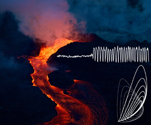
Once this geometry was established, the spillway exhibited intervals of pulsing behaviour characterized by the appearance of large stable oscillations in lava depth and velocity with periods of several minutes (figure 2(a); Patrick et al. Reference Patrick, Dietterich, Lyons, Diefenbach, Parcheta, Anderson, Namiki, Sumita, Shiro and Kauahikaua2019c). Beyond the spillway, the pulsing caused some small overflows of the channel levees that locally widened the flow field. However, most of the upper channelized section of the flow remained more uniform in space and steady in time than the spillway, with little indication of the pulsing behaviour further downstream. The additional ponded storage area at the top of the spillway was clearly hydraulically connected to the cone-bounded pond and spillway, filling and draining during pulsing cycles. Additionally, a second set of cycles was observed (‘surges’) in which the flow from the vent increased significantly over a period of several hours (Patrick et al. Reference Patrick, Dietterich, Lyons, Diefenbach, Parcheta, Anderson, Namiki, Sumita, Shiro and Kauahikaua2019c). These were seen to correspond to large collapse events in the summit caldera, which were inferred to pressurize the subsurface hydraulic connection between the summit and the eruption site. Owing to the strength of this correspondence and explanation for the surges, this paper will focus only on the pulsing oscillations.

Figure 2. (a) Lava level in the spillway at the onset of a pulsing episode from video taken from the spillway monitoring station (Patrick et al. Reference Patrick, Dietterich, Lyons, Diefenbach, Parcheta, Anderson, Namiki, Sumita, Shiro and Kauahikaua2019c). (b) Spectral power (fast Fourier transform, FFT) of pulsing signals in 1-minute real-time seismic-amplitude measurement from station KLUD, and their average (thick dashed black line). The FFT of pulsing in (a) is shown as a thick red line. Each spectrum is denoted by the midpoint time of its pulsing episode. All times are local (HST).
1.1. Pulsing oscillations
From mid-July to the end of the eruption in early August, there were 22 periods of pulsing, identified mainly in infrasound and real-time seismic-amplitude measurement (RSAM), although these may not all be distinct periods (Lyons et al. Reference Lyons, Dietterich, Patrick and Fee2021; figure 2b). Oscillating surface flows are detectable in infrasound due to the acoustic disturbances caused by sloshing and wave breaking. In the volcanological context, changes in vent fountaining activity can also be distinguished in infrasound (Lyons et al. Reference Lyons, Dietterich, Patrick and Fee2021). The RSAM can record the oscillating strength of momentum transfer from shear stresses on the channel base and walls. However, since RSAM is a bulk measurement of all seismic amplitudes at a station, it includes many effects – such as flow through the shallow conduit feeding an eruptive vent, and tremor induced by bubbly flow, as well as noise sources and earthquakes – and is thus only a proxy measurement. Despite this, RSAM spectra yield information about the cyclicity of the pulsing, with most pulsing oscillations exhibiting one of two main bands of periodicity – the stronger band being centred at approximately 6–8 min, with another weaker band centred at approximately 3–4 min (figure 2b). During pulsing episodes, vent fountaining activity was typically anticorrelated with pond and spillway lava level, i.e. fountaining activity greatly increased when the pond level lowered, and greatly decreased when the level raised (Patrick et al. Reference Patrick, Dietterich, Lyons, Diefenbach, Parcheta, Anderson, Namiki, Sumita, Shiro and Kauahikaua2019c). Similarly, infrasound back-azimuth data indicated that the dominant infrasound energy sources also oscillated between the vent (when fountaining was strong, but outflow was slower) and the spillway (when vent fountaining was weaker, and outflow was faster) (Lyons et al. Reference Lyons, Dietterich, Patrick and Fee2021).
These cycles were tentatively assumed to represent variations in vesiculation originating at depth (a forcing on the surface flow dynamics), similar to the phenomenon of ‘gas pistoning’ observed previously at K$\unicode{x012B}$lauea (Swanson et al. Reference Swanson, Duffield, Jackson and Peterson1979; Orr & Rea Reference Orr and Rea2012; Patrick et al. Reference Patrick, Orr, Sutton, Lev, Thelen and Fee2016; Patrick, Swanson & Orr Reference Patrick, Swanson and Orr2019b). Although we will not analyse the gas pistoning mechanism directly in this work, we will give evidence for an alternative hypothesis using a toy model of these oscillations. Here, we posit that the appearance of pulsing is due to a supercritical Hopf bifurcation in the surface fluid dynamics of the pond–spillway system, driven either by an increase in lava supply or a decrease in lava viscosity from the vent. Furthermore, analysis of the fluid dynamics responsible for generating these pulses offers an opportunity to better constrain difficult-to-measure variables such as the viscosity of the lava feeding these hazardous flows.
1.2. Lava fluid dynamic regime
Based on previous studies of the channelized flow from Ahu‘ailā‘au, previous workers have characterized several aspects of the the fluid dynamics of this open channel flow (Patrick et al. Reference Patrick, Dietterich, Lyons, Diefenbach, Parcheta, Anderson, Namiki, Sumita, Shiro and Kauahikaua2019c; Dietterich et al. Reference Dietterich, Diefenbach, Soule, Zoeller, Patrick, Major and Lundgren2021, Reference Dietterich, Grant, Fasth, Major and Cashman2022). Quenched samples taken during the eruption showed that the lava was erupting as a nearly crystal-free mixture of melt and bubbles (as much as 75 % vesicularity). Because of the high gas content, the lava was considerably less dense in the near-vent environment, possibly as little as  $500\unicode{x2013}1300\ {\rm kg}\ {\rm m}^{-3}$ based on vesicularities of 50–82 % (average 70 %) and typical densities of bubble-free basalt. Furthermore, the bulk discharge (or eruption rate) feeding these flows was constrained in the range
  $500\unicode{x2013}1500\ {\rm m}^{3}\ {\rm s}^{-1}$ in a largely rectangular cross-section spillway that was 25–40 m wide. Estimating the viscosity of real lavas is notoriously difficult; however, from the melt's chemistry and empirical rheological models from laboratory studies, the bulk viscosity of the bubbly lava has been estimated in the range
  $O({10^{2}})\unicode{x2013}O({10^{3}})$ Pa s, suggesting a kinematic viscosity
  $O({10^{-1}})\unicode{x2013}O({1})\ {\rm m}^2\ {\rm s}^{-1}$ (Gansecki et al. Reference Gansecki, Lee, Shea, Lundblad, Hon and Parcheta2019; deGraffenried et al. Reference deGraffenried, Hammer, Dietterich, Perroy, Patrick and Shea2021; Soldati, Houghton & Dingwell Reference Soldati, Houghton and Dingwell2021a,Reference Soldati, Houghton and Dingwellb).
Despite the presence of mechanical stirring due to degassing and bubble bursting, undular hydraulic jumps, and breaking oblique shock waves (jumps), the spillway flow during this time was laminar, moving fairly smoothly and lacking self-excited, self-sustaining eddies. In this work, we use a depth-integrated definition of the Reynolds number as
 \begin{equation} Re := \frac{Q}{w\nu}, \end{equation}
where  $Q$ is the bulk discharge,
  $w$ is the channel width, and
  $\nu$ is the bulk kinematic viscosity. Using this definition, the transition to turbulence should occur in the range
  $500 < Re < 2000$ (after Chow Reference Chow1959). Indeed, from previous estimates (Patrick et al. Reference Patrick, Dietterich, Lyons, Diefenbach, Parcheta, Anderson, Namiki, Sumita, Shiro and Kauahikaua2019c; Dietterich et al. Reference Dietterich, Diefenbach, Soule, Zoeller, Patrick, Major and Lundgren2021, Reference Dietterich, Grant, Fasth, Major and Cashman2022), the Reynolds number was approximately in the range
  $50< Re<300$, consistent with the qualitative observation of laminar flow.
Through this period, an undular hydraulic jump and many standing waves were present through the spillway section and to a lesser extent out into the main channel (Dietterich et al. Reference Dietterich, Grant, Fasth, Major and Cashman2022). This implies that the flow leaving the pond was mainly supercritical, characterized by Froude number approximately  $1 < Fr < 1.7$. Estimates of the flow depth from critical flow theories as well as comparisons of syn- and post-eruptive lava surface surveys from unoccupied aircraft systems yield flow depths 3–7 m through much of the spillway (Dietterich et al. Reference Dietterich, Grant, Fasth, Major and Cashman2022). However, the pond was likely much deeper since the final drained and solidified pond surface (at the level of the outflow) is at least 5–10 m above the pre-eruptive surface (inferred to be the bottom of the cone and pond). Downstream of the spillway, the flow slowed and widened considerably, losing all critical flow phenomena. Here, the flow was a wide but channelized viscous gravity current obeying the description of Jeffreys (Reference Jeffreys1925), wherein the depth can be estimated as
 \begin{equation} h\approx \left(\frac{3\nu Q}{w g \tan\beta}\right)^{1/3} ,\end{equation}
where  $\tan \beta$ is the slope of the underlying bed surface, with a remarkably uniform value of approximately
  $0.025$ in this case. Despite the large changes in discharge and stage exhibited by the pulsing, it was clear that the adjustment in flow state was accommodated by the undular hydraulic jump over at least the entire length of the spillway section.
Finally, since typical flow velocities in the spillway were  $5\unicode{x2013}15\ {\rm m}\ {\rm s}^{-1}$, the spillway transit time was considerably less than one minute, thus only a negligible amount of bulk flow cooling was possible before exiting the spillway. We will therefore omit these thermorheological changes and assume an isothermal, isoviscous model.
2. Pond–spillway dynamical model
In this work, we develop a toy model to help explain (in a very simplified way) our proposed mechanism for the generation of pulsing oscillations. It is important to note here that this toy model is intended to be not a high-fidelity representation of the actual dynamics in the pond and spillway, but rather a device for explaining how these oscillations arise in terms of physical effects. This toy system is only complex enough to contain a rather simple Hopf bifurcation with approximately correct waveform and periodicity in a physically realistic range of parameters. Although we could instead study this problem with a richer set of governing equations with less reduction, this simplified approach allows for more targeted interrogation of the oscillatory mechanism at a much lower computational cost.
For this simplified pond–spillway model, we adopt a dynamical systems approach, studying the long-time behaviour of the system (e.g. characterization of attractors, bifurcations) rather than the behaviour of initial transients. Furthermore, because the pulsing phenomenon is primarily temporal (and very slow compared with typical gravity waves), we seek a reduced order model for the system by eliminating explicit spatial dependencies, assuming that a centre manifold (and thus the long-time behaviour) of the pulsing dynamics can be captured with a long-wavelength approach. Much of this paper will focus on analytic and numerical analysis of the phase space of this model from a geometrical or topological perspective, which has become the dominant paradigm in the mathematical study of dynamical systems (e.g. Strogatz Reference Strogatz2015).
For this model, we will analyse the pond depth and exit discharge, assuming that the pond is deeper than the spillway ( $H=H_0+h$), that is, the spillway is fed only by the lava that is above the (constant) base of the outflow (
 $H_0$). We begin by writing a mass balance for the pond, including some effect of compressibility owing to the high vesicularity of the erupted lava (
 $\phi \sim 0.7$):
 \begin{equation} \frac{1}{\rho}\,{\frac{{\rm d} }{{\rm d} t}}(\rho H) = \frac{1}{A}\,(Q_0-Q) , \end{equation}
where  $Q_0$ is the bulk volumetric eruption rate (assumed constant),
  $Q$ is the bulk discharge out of the pond, and
  $A$ is the area of the pond surface which varied between
  $6500< A<8500\ {\rm m}^2$.
In this work, we treat the ponded lava as a bulk compressible medium with an isothermal equation of state  $\rho = \rho (\,p)$. Furthermore, we assume that the balance of vertical momentum reduces to a hydrostatic form for the bulk pressure
  $p =k \rho g H$, where
  $k$ is a constant of proportionality reflecting the relative depth in the pond where the bulk pressure is acting most to compress the mass (e.g.
  $k=1/2$ for the depth-averaged pressure). Although this sets up an implicit relationship for the bulk density, we can rewrite the left-hand side of (2.1) as
 \begin{equation} \frac{1}{\rho}\,{\frac{{\rm d} }{{\rm d} t}}(\rho H) = {\frac{{\rm d} H}{{\rm d} t}} + H\,\frac{1}{\rho}\,{\frac{{\rm d} \rho}{{\rm d} t}} = {\frac{{\rm d} H}{{\rm d} t}} + H\,\frac{1}{\rho}\,{\frac{{\rm d} \rho}{{\rm d} p}}\,{\frac{{\rm d} p}{{\rm d} t}} = {\frac{{\rm d} H}{{\rm d} t}} + kgH\,{\frac{{\rm d} \rho}{{\rm d} p}}\,\frac{1}{\rho}{\frac{{\rm d} }{{\rm d} t}}(\rho H), \end{equation}
from which we can write
 \begin{equation} {\frac{{\rm d} H}{{\rm d} t}} = \left( 1 - kgH\,{\frac{{\rm d} \rho}{{\rm d} p}}\right)\frac{1}{\rho}\,{\frac{{\rm d} }{{\rm d} t}}(\rho H)= \left( 1 - kgH\, {\frac{{\rm d} \rho}{{\rm d} p}}\right) \frac{1}{A}\,(Q_0-Q). \end{equation}
Now we must deal with the term in parentheses, which we address by computing the bulk compressibility, assuming that all of the bulk compressibility is accommodated by a constant mass of isothermal ideal gas in a dispersed bubble phase:
 \begin{align} \frac{1}{\rho}\,{\frac{{\rm d} \rho}{{\rm d} p}} &=-\frac{1}{V}\,{\frac{{\rm d} V}{{\rm d} p}} =-\frac{1}{V} \left({\frac{{\rm d} V^{gas}}{{\rm d} p}}+{\frac{{\rm d} V^{lava}}{{\rm d} p}}\right) \approx-\frac{1}{V}\,{\frac{{\rm d} V^{gas}}{{\rm d} p}} \nonumber\\ &=-\frac{n R T}{V}\,{\frac{{\rm d} }{{\rm d} p}}\left(\frac{1}{p}\right) = \frac{n R T}{V p^2} = \frac{V^{gas}}{V}\,\frac{1}{p} = \frac{\phi}{p}. \end{align}
On substituting, we obtain
 \begin{equation} {\frac{{\rm d} H}{{\rm d} t}} = \frac{1 - \phi}{A}\,(Q_0-Q). \end{equation}
In this simplified view of the pond, compressibility of the lava from the presence of vesicles limits the rate of change of the pond since some fraction of these changes is either compressed or expanded as mass (and weight) is either added to or removed from the pond.
As the lava exits the pond into the spillway, the Saint-Venant equations in a rectangular channel of uniform width provide a reasonable first-order approximation to the conservation of momentum for a shallow, long-wavelength flow:
 \begin{equation} \partial_t q + \partial_x\left(\frac{q^2}{\eta} + \frac{1}{2}\,g\eta^2\right)= g\eta \tan\beta - \frac{\tau}{\rho} , \end{equation}
where  $q(x,t)$ and
  $\eta (x,t)$ are the discharge per unit width and the depth, respectively, and
  $\tau$ is the basal shear stress. To match the conditions at the pond exit, we have that
  $w q|_{exit} = Q$ and
  $\eta |_{exit} = H-H_0 = h$.
Because the pond volume depends mainly on broad scale changes in the outflow, we will consider only long-wavelength spatial changes so as to capture the overall slow discharge changes in the flow system. Towards this end, we seek to generate a lumped-element momentum model from (2.6), requiring approximation of the spatial derivatives. First, we treat the spatial derivative in the convective term as a finite difference over a baseline ( $L$, of the order of the spillway length) over which long-wave variations in momentum flux (
 $q^2/\eta$) decay:
 \begin{equation} \left.\partial_{x}\left(\frac{q^2}{\eta}\right)\right|_{exit} \approx \frac{1}{L}\left(\left.\frac{q^2}{\eta}\right|_{L}-\left.\frac{q^2}{\eta}\right|_{exit}\right)= \frac{1}{L}\left(\frac{Q_L^2}{ w^2 h_L}-\frac{Q^2}{ w^2h}\right)\!, \end{equation}
where  $Q_L$ and
  $h_L$ are the downstream discharge and depth (assuming constant channel width down the spillway). This approximation is equivalent to modelling the momentum flux decaying to a background (constant) value far downstream:
 \begin{equation} \frac{q^2}{\eta} \approx \left.\frac{q^2}{\eta}\right|_{L} + \left(\left.\frac{q^2}{\eta}\right|_{exit}-\left.\frac{q^2}{\eta}\right|_{L}\right)\exp\left(-\frac{x}{L}\right), \end{equation}
which predicts that the anomalous momentum flux has almost completely decayed by  $x>2L$. This phenomenological model is based on the observation that further downstream, critical flow phenomena were largely absent, and the Reynolds number is much decreased due to the wider channel, suggesting that the lava flow is no longer driven by inertial forces, thus the convective terms can be neglected there. In this work, we estimate
  $250< L<350$ m based on the approximate length of the spillway and the pattern of velocity decay measured by Dietterich et al. (Reference Dietterich, Grant, Fasth, Major and Cashman2022). Although we do not include diffusion terms here, longitudinal momentum diffusion and dissipation due to mixing likely help to enforce this decay in the real flow (as in the eddy viscosity closure, e.g. Elder Reference Elder1959; Wu, Wang & Chiba Reference Wu, Wang and Chiba2003).
As a consequence of the long-wavelength approximation, we will also assume that the average pressure gradient is dominated by the underlying slope rather than changes in depth, and thus will neglect the  $\partial _x(\tfrac {1}{2}g\eta ^2)$ term. Indeed, this quantity was small over long baselines in the real flow (Dietterich et al. Reference Dietterich, Grant, Fasth, Major and Cashman2022). If we were to retain this term and treat it with a similar phenomenological model as the momentum flux, the there would be little impact on the reduced-order dynamical system except to include additional parameters (see Appendix A).
Finally, we require an estimate of the resisting bed shear stress. For a laminar flow, the bed shear stress in a wide rectangular open channel will take the form
 \begin{equation} \frac{\tau}{\rho} \sim \frac{1}{8}\times \frac{24}{Re} \times \left|\frac{Q}{w h}\right|\frac{Q}{w h} = 3\nu\,\frac{Q}{w h^2}. \end{equation}
It is important to note that although we are considering only laminar flow, a transitional friction model would be necessary for higher flow rates. This would provide significantly enhanced resistance for high Reynolds numbers compared with a laminar-only model.
Recalling that the geometry of the pond exit gives  ${{{\rm d} H}/{{\rm d} t}} = {{{\rm d} h}/{{\rm d} t}}$, the resulting toy dynamics for the pond system can be written as a
  $2\times 2$ system:
 \begin{gather} {\frac{{\rm d} h}{{\rm d} t}} = \dfrac{1-\phi}{A}\,(Q_0-Q), \end{gather}
 \begin{gather} {\frac{{\rm d} Q}{{\rm d} t}} = gwh\tan\beta - 3\nu\,\dfrac{Q}{h^2} + \dfrac{1}{w L}\left(\dfrac{Q^2}{ h} - \dfrac{Q_L^2}{ h_L}\right). \end{gather}
For the remainder of this paper, we will focus on analysing a dimensionless form of this system, using the non-dimensionalization
 \begin{equation} \mathcal{T} := 3\nu t / h_c^2,\quad \mathcal{H}(\mathcal{T}) := h(t)/h_c,\quad \mathcal{Q}(\mathcal{T}) := Q(t)/Q_0, \end{equation}
where the depth scaling  $h_c := (3\nu Q_0 / gw\tan \beta )^{1/3}$ is the flow depth predicted for the laminar kinematic wave solution to the Saint-Venant equations and is equivalent to that predicted by Jeffreys equation (Jeffreys Reference Jeffreys1925; Dietterich et al. Reference Dietterich, Grant, Fasth, Major and Cashman2022). This yields the following dimensionless planar dynamical system (with
  $\dot {(\;\;)}\equiv {{{\rm d} }/{{\rm d} \mathcal {T}}}$ from here onwards):
 \begin{gather} \dot{\mathcal{H}} = a(1-\mathcal{Q}), \end{gather}
 \begin{gather} \dot{\mathcal{Q}} = \mathcal{H} - \dfrac{\mathcal{Q}}{\mathcal{H}^2} + b \left(\dfrac{\mathcal{Q}^2}{\mathcal{H}} - c\right), \end{gather}
where we have defined the dimensionless quantities
 \begin{gather} a := (1-\phi){Q_0 h_c}/{3\nu A}, \end{gather}
 \begin{gather} b := {Q_0 h_c}/{3\nu w L}, \end{gather}
 \begin{gather} c: = Q_L^2 h_c / Q_0^2 h_L. \end{gather}
 In this work, we will make use of several alternative parametrizations of the parameters  $a$ and
  $b$. By introducing
  $\sigma = (1-\phi )w L / A$, we can write
  $a = \sigma b$ in the pond height equation, highlighting the mutual dependence of both
  $a$ and
  $b$ on the outflow depth and discharge. In this parametrization,
  $\sigma$ is related principally to where lava is stored, measuring the ratio of the flow surface area in the spillway to the pond area corrected for the compressibility of the deeper ponded lava. An additional physics-based parametrization can be made by first introducing an overall Reynolds number for the eruption rate
  $Re_0 = Q_0/w\nu$, and another parameter
  $\gamma = (\nu ^2/9L^3g\tan \beta )^{1/3}$ describing the dimensionless pressure gradient or drop along the channel (related to the Hagan or Bejan numbers; e.g. Awad Reference Awad2013). We can then recast both parameters as powers of the Reynolds number,
 \begin{equation} \begin{pmatrix}{a}\\{b} \end{pmatrix} = \begin{pmatrix}{\sigma}\\ {1}\end{pmatrix} \gamma\,Re_0^{4/3}, \end{equation}
highlighting the fact that these parameters are related primarily to the amount of inertia relative to friction. We will only use this parametrization later when considering (briefly) a laminar–turbulent transitional friction model.
Although our model has three parameters, we will hereon take  $c=1$, following the logic that the overall lava flow system, from vent to sections further downstream, is in equilibrium even if there can be transient dynamics in the pond and spillway. To see this, consider the system when the convective term can be neglected, which is an appropriate omission far downstream (taking
  $b\rightarrow 0$):
 \begin{gather} \dot{\mathcal{H}} = a(1-\mathcal{Q}), \end{gather}
 \begin{gather} \dot{\mathcal{Q}} = \mathcal{H} - {\mathcal{Q}}/{\mathcal{H}^2}. \end{gather}
This system admits only one fixed point,  $\mathcal {H}=\mathcal {Q}=1$, which corresponds to steady flow in which the discharge exactly matches the eruption rate, and the depth is given by the Jeffreys equation. In this case, where the system is not only laminar, but essentially Stokesian with transient relaxation, the equilibrium is globally stable (Appendix B). The interpretation of this stable equilibrium is that downstream, where inertial forces are no longer significant, the system evolves towards that given by Jeffreys (Reference Jeffreys1925), thus the downstream background value for the momentum flux is approximately
  $Q_0^2/w^2 h_c$. As a consequence, with
  $c=1$, this equilibrium point is preserved and is invariant to changes in
  $a$ and
  $b$; however, it will not always be a stable equilibrium, as we will show. Intuitively, this choice of finite-difference end condition prevents continuous overfilling or depletion of the spillway and greater lava flow system over time. We assert here, without proof, that taking
  $c\neq 1$ (but within a plausible range) does not significantly affect the dynamics of the system, or our conclusions.
It is important to note here that we have made significant approximations to arrive at such a simple system without spatial dependence. In general, better approximations will contain additional parameters as well as a more complete basal friction model that includes lateral wall stress or captures the laminar–turbulent transition. However, our system is the simplest conceivable dynamical system that contains a gravitational driving force, depth-dependent basal shear stress, and the effects of convective accelerations (inertia).
2.1. Stability of equilibria
Here, we analyse the simplified system
 \begin{gather} \dot{\mathcal{H}} = a(1-\mathcal{Q}), \end{gather}
 \begin{gather} \dot{\mathcal{Q}} = \mathcal{H} - \dfrac{\mathcal{Q}}{\mathcal{H}^2} + b\left(\dfrac{\mathcal{Q}^2}{\mathcal{H}} - 1\right), \end{gather}
with physically realistic values  $a>0$ and
  $b>0$ in the right half-plane (
 $\mathcal {H}>0$). All equilibria of this system can be found at the intersections of the
  $\dot {\mathcal {H}}$ nullcline (
 $\mathcal {Q}=1$) and the
  $\dot {\mathcal {Q}}$ nullcline:
 \begin{equation} \mathcal{Q} = \mathcal{N}^\pm_b(\mathcal{H}) = \frac{1}{2b\mathcal{H}}\pm\sqrt{\frac{1}{4b^2\mathcal{H}^2}+\mathcal{H}\left(1-\frac{\mathcal{H}}{b}\right)} . \end{equation}
For  $b<3$, there is only one fixed point,
  $\mathcal {H}=\mathcal {Q}=1$, which has the following eigenvalues:
 \begin{equation} \lambda_\pm= b-\tfrac{1}{2} \pm i\, \sqrt{(3-b)a - \left(b-\tfrac{1}{2}\right)^2}.\end{equation}
These eigenvalues are a pair of complex conjugates for  $(3-b)a - (b-{1}/{2})^2>0$. Outside this range, the spiral breaks down, resulting in a stable or unstable node depending on whether
  $b$ is below or above this range, respectively (figure 3a). At
  $b=3$, a pitchfork bifurcation occurs, producing two additional unstable equilibria at
  $\mathcal {H} = \mathcal {H}_\pm = \tfrac {1}{2}(b-1)\pm \tfrac {1}{2}\sqrt {(b+1)(b-3)}$ (figure 3b).

Figure 3. (a) Real and imaginary parts of the eigenvalues (solid and dashed, respectively) of the three equilibria (with  $\sigma = 1$). Colours correspond to equilibria at
  $(1,1)$ (black),
  $(\mathcal {H}_+,1)$ (cyan) and
  $(\mathcal {H}_-,1)$ (magenta). Vertical lines mark the Hopf (black) and pitchfork (green) bifurcations, as well as the transition from unstable node to unstable spiral for
  $(\mathcal {H}_+,1)$ (cyan) and
  $(\mathcal {H}_+,1)$ (magenta). (b) Nullclines of
  $\dot {\mathcal {H}}$ (blue) and
  $\dot {\mathcal {Q}}$ (red) near the pitchfork bifurcation. Equilibria are colour-coded as in (a). Semi-transparent plane is
  $\mathcal {Q} = 1$. (c) Schematic flow near the slow manifold (green) after the pitchfork (
 $b=3.5$, yellow-shaded slice in b). Unstable manifolds are dashed. Trajectories are shown schematically (black).
At the pitchfork, the slower unstable eigenvector of the main fixed point reverses direction, and  $(\mathcal {H},\mathcal {Q})=(1,1)$ transitions from an unstable node to a saddle. Here, the two nullclines become tangent at
  $(1,1)$, with
  $\mathcal {Q} = \mathcal {N}^+_b(\mathcal {H})$ remaining close to
  $\mathcal {Q}=1$ between the new fixed points (
 $\mathcal {H}_-\leq \mathcal {H}\leq \mathcal {H}_+$). As a consequence, the dynamics become very slow along the
  $\dot {\mathcal {Q}}$ nullcline compared with the dynamics along the unstable manifolds of the fixed points (figure 3c). Indeed, just past the pitchfork, each (real) equilibrium has a near-zero eigenvalue, with the other (real) eigenvalue separated from it by a spectral gap, thus producing the slow dynamics (figure 3a). Informally, a centre (slow) manifold exists very close to the nullcline, producing reduced dynamics that can be modelled approximately by substituting (2.17) into (2.16a):
 \begin{equation} \dot{\mathcal{H}} = a\left(1-\mathcal{N}^+_b(\mathcal{H})\right)\!. \end{equation}
From the sign of this approximation, the pitchfork is subcritical: the main unstable node gains stability (in this subspace only), and two unstable nodes are created. However, because the three fixed points are strongly repelling in every direction other than along the slow subspace, this reduced dynamics is not physically realizable in the presence of noise. Consequently, we will focus the remainder of this study on the main fixed point at  $\mathcal {H}=\mathcal {Q}=1$, in the near neighbourhood of
  $b=\tfrac {1}{2}$ where a Hopf bifurcation occurs.
2.2. Hopf bifurcation
The Andronov–Hopf bifurcation (hereon, Hopf bifurcation) is the simplest bifurcation involving periodic solutions, requiring only one condition (and thus only one parameter) (e.g. Guckenheimer & Holmes Reference Guckenheimer and Holmes1983; Strogatz Reference Strogatz2015). Hopf bifurcations occur as local phenomena when a complex conjugate pair of eigenvalues of a fixed point passes through the imaginary axis ( ${\rm Re} (\lambda _\pm ) =0$), either gaining or losing stability. In this system, the equilibrium loses stability for
  $b>\tfrac {1}{2}$ (figure 3a). Trivially, since the eigenvalues cross the bifurcation point with non-zero rate (
 ${\rm d}\lambda _\pm /{\rm d}b > 0$ at
  $b=\tfrac {1}{2}$), the bifurcation is not degenerate and a small limit cycle is excited. Because the vector field away from the small limit cycle is still spiraling inwards, this is an example of a supercritical Hopf bifurcation. This can be verified by constructing a trapping region, out of which no trajectories can escape (Appendix B).
2.3. Pond outflow oscillator
The oscillator in this system is due to two primary factors: inertia of the outflow and strongly depth-dependent frictional resistance. If there exists a pond lava height in excess of that needed to maintain inflow–outflow equilibrium, then the outflow discharge will increase as the gravitational driving force increases. Eventually, the discharge exceeds the eruption rate and the pond begins to drain, while the pond outflow continues to increase due to a combination of continued excess gravitational force and convective acceleration (due to inertia). As the pond level falls, the outflow bed resistance increases significantly as  $O({1/\mathcal {H}^2})$, which eventually becomes large enough to arrest and reverse the increasing trend in discharge. Eventually, the discharge falls below the pond inflow rate and the pond begins to refill again, significantly decreasing the impact of basal friction on the flow, allowing acceleration the outflow discharge once again. As shown in figure 4, at higher values of
  $b$, these cycles are stronger, producing larger spikes in discharge and much faster collapses. This leads from a small amplitude oscillator to a two-stroke relaxation oscillator (e.g. Jelbart & Wechselberger Reference Jelbart and Wechselberger2020).

Figure 4. Summary of the Hopf bifurcation for  $a=1.0$. (a–c) Phase portraits for three values (0.4, 0.5, 0.6) of the parameter
  $b$ showing the flow (grey), example orbits (magenta), the limit cycle (bold, black), the
  $\mathcal {H}$ and
  $\mathcal {Q}$ nullclines (blue and red dashed, respectively). Equilibrium stability indicated by marker fill. (d) Same as (c), colour-coded by local cycle speed
  $\sqrt {\dot {\mathcal {H}}^2+\dot {\mathcal {Q}}^2}$. (e) Dependence of the limit cycle on
  $b$. (f) Bifurcation diagram showing the
  $\mathcal {H}$ and
  $\mathcal {Q}$ cycle extrema (blue and red, respectively), the stable node (black), and the unstable node (dashed black). (g) Comparison of cycle-averaged radius from averaging theory (magenta) and numerical integration (green dots).
Although analyses exist for relaxation oscillators by singular perturbation methods (e.g. Stoker Reference Stoker1950; Strogatz Reference Strogatz2015; Jelbart & Wechselberger Reference Jelbart and Wechselberger2020), these require the existence of a small parameter multiplying one of the time derivatives, which is not the case here. In this system, the  $O({1/\mathcal {H}^2})$ friction induces the relaxation phase rather than a small constant parameter. The
  $\dot {\mathcal {Q}}$ equation is only periodically singular (owing to the factor
  $\mathcal {H}^{-2}$), which is a much more difficult case. We restrict this work to analysing the small-amplitude limit of the oscillations just past the Hopf bifurcation.
2.3.1. Small-amplitude oscillator
When combined, the planar system can be written as a damped, nonlinear oscillator with a nonlinear restoring force, and nonlinear rate- and state-dependent damping:
 \begin{equation} \ddot{\mathcal{H}} =-a\left(\mathcal{H}-\frac{1}{\mathcal{H}^2}-b\left(1-\frac{1}{\mathcal{H}}\right)\right) + \left(2b-\frac{1}{\mathcal{H}} - \frac{b}{a}\, \dot{\mathcal{H}}\right)\frac{\dot{\mathcal{H}}}{\mathcal{H}}. \end{equation}
When linearized for small deviations  $X= \mathcal {H}-1$ about the equilibrium point, this becomes the familiar linear damped harmonic oscillator:
 \begin{equation} \ddot{X} =-a(3-b)X + (2b-1)\dot{X} \end{equation}
where the negative damping  $2b-1$ demonstrates the localized effect of the Hopf bifurcation. Exactly at the bifurcation (
 $b=\tfrac {1}{2}$), a small-amplitude (
 $\varepsilon \ll 1$) periodic orbit is born:
 \begin{gather} \mathcal{H} = 1 + \varepsilon \cos\left(\sqrt{a(3-b)}\,(\mathcal{T}+\varphi_0)\right), \end{gather}
 \begin{gather} \mathcal{Q} = 1 + \varepsilon\,\sqrt{\frac{3-b}{a}}\sin\left(\sqrt{a(3-b)}\,(\mathcal{T}+\varphi_0)\right), \end{gather}
for an arbitrary initial phase  $\varphi _0$. Using this basic solution, we can extend this analysis past the Hopf bifurcation while retaining the nonlinearities. To do this, we will convert to polar coordinates and then assume that the radius and phase are slowly varying functions of time compared with the period of the main oscillation (
 $2{\rm \pi} /\sqrt {a(3-b)}$).
2.3.2. Averaging theory
To analyse how the limit cycle changes near the bifurcation, we use a form of averaging theory in polar coordinates (Guckenheimer & Holmes Reference Guckenheimer and Holmes1983; Strogatz Reference Strogatz2015). First, we define the radius  $r(\mathcal {T})$ and phase
  $\varphi (\mathcal {T})$ implicitly via
 \begin{gather} \mathcal{H}(\mathcal{T}) = 1 + r(\mathcal{T})\cos\left(\sqrt{a(3-b)}\,(\mathcal{T}+\varphi(\mathcal{T}))\right), \end{gather}
 \begin{gather} \mathcal{Q}(\mathcal{T}) = 1 + \sqrt{\frac{3-b}{a}}\,r(\mathcal{T})\sin\left(\sqrt{a(3-b)}\,(\mathcal{T}+\varphi(\mathcal{T}))\right)\!. \end{gather}
Substituting the above definitions for the radius and phase into the  $\mathcal {H},\mathcal {Q}$ system, differentiating, and rearranging results in a polar form of the radial equation, gives
 \begin{align} \dot{r} &= \frac{r}{(1+rC)^2}\left\{2\left(b-\frac{1}{2}\right)S^2 + r\left[2bS^2C - \sqrt{a(3-b)}\,S C^2+\sqrt{\frac{3-b}{a}}\,b S^3\right]\right.\nonumber\\ &\quad \left.{}+r^2 \left[\sqrt{\frac{a}{3-b}}\,(b-2)SC^3+\sqrt{\frac{3-b}{a}}\,bS^3C\right]\right\}, \end{align}
where we have used the shorthand  $C = \cos \theta$ and
  $S = \sin \theta$, with
  $\theta = \sqrt {a(3-b)} \,\times $ $(\mathcal {T}+\varphi (\mathcal {T}))$. The equivalent expression for the phase can be found from
 \begin{equation} \dot{\varphi} = \frac{1}{\sqrt{a(3-b)}}\,\frac{C}{S}\,\frac{\dot{r}}{r}. \end{equation}
From (2.24) and (2.25), we can readily see that just past the Hopf bifurcation ( $0< b-\tfrac {1}{2}\ll 1$), where
  $r\ll 1$, the radius and phase are both slowly varying functions of time. In this restriction, the slow variation of the radius and phase are negligible on the time scale of the main oscillations, thus the averaging approximation (for an average over the
  $\mathcal {P}$-periodic fast-time oscillations) can be written as
 \begin{align} {\left\langle\, f\right\rangle} &:= \frac{1}{\mathcal{P}}\int_{\mathcal{T}}^{\mathcal{T}+\mathcal{P}}f\left(C(s), S(s), r(s)\right){\mathrm{d}s}\nonumber\\ &\approx \frac{1}{\mathcal{P}}\int_{\mathcal{T}}^{\mathcal{T}+\mathcal{P}}f\left( \cos\left[\sqrt{a(3-b)}\left(s+{\left\langle\varphi\right\rangle}\right)\right]\!, \sin\left[\sqrt{a(3-b)} \left(s+{\left\langle\varphi\right\rangle}\right)\right]\!, {\left\langle r\right\rangle}\right){\mathrm{d}s}\nonumber\\ &=\frac{1}{2{\rm \pi}}\int_{0}^{2{\rm \pi}}f\left(\cos\theta,\sin\theta, {\left\langle r\right\rangle}\right){\mathrm{d}\theta}. \end{align}
 If we expand (2.24) and (2.25) in Taylor series up to  $O(r^3)$, average over the fast-time cycles and develop a solution in a small parameter
  $\delta ^2 = b-\tfrac {1}{2}\ll 1$ as
  ${\left \langle r (\mathcal {T})\right \rangle } = \delta R(\mathcal {T})$, then we can recover the supercritical Hopf normal form (e.g. Strogatz Reference Strogatz2015) for this system:
 \begin{gather} \dot{R}= \delta^2 R \left(1 - \frac{R^2}{4}\right) + O(\delta^4), \end{gather}
 \begin{gather} \dot{\varphi}= \delta^2 R^2\left(\frac{21}{40} - \frac{1}{16a}\right) + O(\delta^4). \end{gather}
From the normal form, we can see that the evolution progresses from an initial  $R_0$ as
 \begin{equation} R(\mathcal{T}) = \frac{2\exp(\delta^2 \mathcal{T})}{\sqrt{(2 R_0)^{-2} - 1 + \exp(2 \delta^2 \mathcal{T})}}, \end{equation}
approaching  $R\rightarrow 2$ on time scales of
  $O(1/\delta ^2)$. This produces a cycle-averaged radius of
 \begin{equation} {\left\langle r\right\rangle} \rightarrow 2 \delta = 2\sqrt{b-\tfrac{1}{2}},\end{equation}
which compares well with the numerical solution (figure 4g).
One interesting aspect of this analysis in comparison to the numerical integration is that as  $b$ grows, the maximum amplitude of the oscillations grows very quickly, exhibiting large, positive departures in discharge (figure 4e,f). However, the cycle-averaged radius grows much more modestly. This suggests that these large-amplitude cycle segments occur more quickly the larger they grow, shortening in duration faster than their amplitude grows so that, overall, the cycle-averaged radius grows slowly. Though intriguing, the ultimate fate of the limit cycle as
  $b$ grows large is beyond the scope of this work.
3. Comparison with 2018 K $\unicode{x012B}$lauea eruption
Since measuring the lava level cycles was possible only in the spillway, our model of the onset of these cycles in the pond is not directly comparable to the measurements. To make this comparison, we must investigate how the periodic forcing from the pond is changed on its way to the measurement location in the spillway. Here, we reduce the dimensionality of the spillway dynamics by considering a weighted average of the the downstream flow behaviour using the following weighted Reynolds operator appropriate for semi-infinite domains:
 \begin{equation} \bar{\varphi}(t) := \int_0^\infty \varphi(x,t)\,\frac{1}{L}\exp\left(-\frac{x}{L}\right) {\mathrm{d}\kern 0.06em x} \end{equation}
for some bounded function  $\varphi (x,t)$. By inspection, we can see that this is a linear operator that commutes with the time derivative, whereas the weighted average of
  $x$-derivatives can be obtained from integration by parts, yielding the relation
 \begin{equation} \overline{\partial_{x}\varphi} = \frac{\bar{\varphi}-\varphi|_{x=0}}{L}. \end{equation}
This allows us to rewrite the Saint-Venant system for the forced spillway as
 \begin{gather} {\frac{{\rm d} \bar{\eta}}{{\rm d} t}} = \frac{1}{w L}\left(Q(t) - w\bar{q}\right), \end{gather}
 \begin{gather} {\frac{{\rm d} \bar{q}}{{\rm d} t}} = g\bar{\eta}\tan\beta - 3\nu\,\frac{\bar{q}}{\bar{\eta}^2} + \frac{1}{w^2 L}\left(\frac{Q^2(t)}{ h(t)} - \frac{w^2\bar{q}^2}{\bar{\eta}}\right)\!, \end{gather}
where terms with explicit time dependence are the solutions of the pond system which act as a forcing. In this averaging, we have made the approximation that the average of products is the product of averages. This approximation introduces errors when spatial fluctuations are large and in-phase compared with the averaged quantities. In typical Reynolds-averaged theories in fluid dynamics (e.g. Reynolds-averaged Navier–Stokes; Chou Reference Chou1945), the averages of these terms induce additional stresses due to cross-correlation of fluctuations; however, these terms are expected to be quite small here since observed spatial fluctuations in the spillway were substantially smaller than their mean values (Dietterich et al. Reference Dietterich, Grant, Fasth, Major and Cashman2022).
The non-dimensional version of this system depends solely on the parameter  $b$:
$b$:
 \begin{gather} \dot{\mathcal{H}}_s = b\left(\mathcal{Q}(\mathcal{T}) - \mathcal{Q}_s\right), \end{gather}
 \begin{gather} \dot{\mathcal{Q}}_s = \mathcal{H}_s - \frac{\mathcal{Q}_s}{\mathcal{H}_s^2} + b\left(\frac{\mathcal{Q}^2(\mathcal{T})}{\mathcal{H}(\mathcal{T})} - \frac{\mathcal{Q}_s^2}{\mathcal{H}_s}\right)\!, \end{gather}
where  $\mathcal {H}_s = \bar {\eta }/h_c$ and
  $\mathcal {Q}_s = w\bar {q}/Q_0$ are, respectively, the average spillway depth and discharge, non-dimensionalized in the same way as the pond system ((2.16a), (2.16b)), which now plays the role of an oscillatory forcing.
Importantly, without an oscillatory forcing from the pond, there cannot be any self-excited oscillation in the spillway. This can be seen by examining the effect of taking the pond forcing to be constant in time (most appropriately,  $\mathcal {H}=\mathcal {Q} \equiv 1$) for the spillway system. For the steadily forced spillway, a stable fixed point will exist at
  $\mathcal {H}_s=\mathcal {Q}_s = 1$ for all
  $b>0$. Its eigenvalues can be found by sending
  $b\mapsto -b$ and
  $a\mapsto b$ in (2.18) (the pond system eigenvalues):
 \begin{equation} (\lambda_s)_\pm=-\left(b+\tfrac{1}{2}\right) \pm{\rm i}\,\sqrt{(3+b)b - \left(b+\tfrac{1}{2}\right)^2}, \end{equation}
which have negative real parts for all  $b>0$, and thus local asymptotic stability. Additionally, the global stability of this fixed point can be demonstrated by a logic similar to the arguments for the pond system (Appendix B), except that here, the
  $\dot {\mathcal {Q}}_s$ nullcline has only a single branch in the first quadrant,
 \begin{equation} \mathcal{Q}_s = \mathcal{N}^+_{-b}(\mathcal{H}_s), \end{equation}
which is monotone for all  $b>0$, going asymptotically to the line
  $\mathcal {Q}_s \sim \mathcal {H}_s/\sqrt {b} + \sqrt {b}/2$ for large depth. This enables easy construction of trapping regions of arbitrarily large size in the first quadrant. Furthermore, the local convergence rate of perturbations to the equilibrium point gets stronger for larger values of
  $b$. All of this together means that sustained, distinctly observable pulsing in the spillway requires a substantial periodic forcing from the pond, without which the spillway dynamics would decay very quickly.
Solutions to the forced spillway system behave similarly to the pond, highlighting the rapid convergence of the spillway system to the pond forcing (figure 5a). However, one critical difference is that the spillway depth and discharge are more closely co-varying than in the pond, creating an elongated cycle in phase space that agrees well with the spillway pulsing data of Patrick et al. (Reference Patrick, Dietterich, Lyons, Diefenbach, Parcheta, Anderson, Namiki, Sumita, Shiro and Kauahikaua2019c); see figure 5(b). Indeed, this toy model gives an accurate prediction of the depth and discharge waveforms in both their asymmetry and phase, with the discharge lagging slightly behind the depth, although this lag is somewhat smaller in the observed pulsing data (figures 5c,d). For the pulsing data in figure 5, the best fitting value of  $b$ is just past the Hopf bifurcation in
  $0.52< b<0.55$, indicating that the small-amplitude oscillator approximation is realistic.

Figure 5. Pond limit cycle forcing on spillway dynamics using the parametrization  $a=\sigma b$ with
  $\sigma =0.4$. (a) Limit cycles for various values of the parameter
  $b$ showing the pond cycles (dotted) and the resulting forced cycles in the spillway (solid). (b) Forced spillway cycles for values of
  $b$ bracketing the pulsing data of Patrick et al. (Reference Patrick, Dietterich, Lyons, Diefenbach, Parcheta, Anderson, Namiki, Sumita, Shiro and Kauahikaua2019c). Grey bars represent measurement error. (c) Spillway cycle waveform (
 $b=0.515$) for comparison with (d) depth and discharge data. All data are scaled using
  $Q_0=1000\ {\rm m}^{3}\ {\rm s}^{-1}$ and
  $h_c=5.5$ m.
3.1. Cycle periodicity
Because the pulsing data are well explained by a small-amplitude oscillator in the vicinity of the Hopf bifurcation, we may estimate the predicted value of the cycle period ( $P$) as that occurring right at the Hopf bifurcation (
 $b=1/2$):
 \begin{equation} P = \left.\frac{h_c^2}{3\nu}\,\frac{2{\rm \pi}}{\sqrt{a(3-b)}}\right|_{b={1}/{2}} = 2{\rm \pi}\,\sqrt{\frac{A}{2.5(1-\phi)gw\tan\beta}}, \end{equation}
which can be seen to include mainly geometric factors of the pond and spillway as well as the vesicularity of the erupting lava. Using pond areas  $6500\unicode{x2013}8500\ {\rm m}^2$, a spillway width 25–40 m, spillway slope 0.025 (1 m drop per 40 m run), and vesicularity 50–82 % yields a cycle of period 2.4–5.8 min, which is in line with the shorter of the two observed periodicities (in figure 2b). If the additional ponded storage area (figure 1,
  ${\sim }4500\ {\rm m}^2$) is included (i.e. it fills and empties in hydraulic connection with the main cone-bounded pond), then this lengthens to 3.1–7.2 min, which for the high end is consistent with the slower oscillation. Although it is difficult to compare the periodicity precisely owing to variations in the measured parameters, the spectrum of predicted periodicities generally agrees well with those observed.
4. Discussion
The central hypothesis of this work is that the pulsing activity seen during the eruption was due to intermittent crossing of a Hopf bifurcation in the fluid dynamics of the ponded storage region and its outflow. Although the oscillations in pond level were not measurable directly due to volcanic gases and proximal volcanic hazards, the pond cycles acted as an oscillating forcing on the spillway dynamics, which was more easily measured. As demonstrated above, the limit cycles generated by this bifurcation are comparable in waveform and periodicity to those measured in the spillway during the eruption. Because the Hopf bifurcation controlling parameter  $b$ is related to the Reynolds number via the eruption rate and viscosity, we assert that the pulsing regimes were the result of slow (and modest) changes in these quantities, that is, either an increase in eruption rate or a decrease in viscosity. Although our hypothesis suggests that such changes can start or stop pulsing, explanations for slow and intermittent variability in these quantities, as well as the relationship between the pulsing and surging behaviour, are beyond the scope of this work.
Although this model of pond–spillway oscillation is in good agreement with the observed pulsing oscillations, in the next subsection, we will address the hypothesis that the oscillations are forced directly by shallow degassing processes. Additionally, we will further discuss a few deficiencies of the proposed mathematical model. Specifically, we will consider its tendency to produce (potentially unphysical) large-amplitude limit cycles for modest values of  $a$ and
  $b$, and how the choice of friction regime (laminar or turbulent) influences these dynamics. Finally, we will use the analysis of the Hopf bifurcation to estimate the viscosity of the erupted lava, a parameter relevant to broader lava hazard modelling efforts.
4.1. Oscillating gas forcing hypotheses
The hypothesis adopted during and directly after the eruption was that the pulsing behaviour was the direct result of variation in the amount of gas erupting from the vent, causing an oscillating supply of bulk vesiculated lava from depth. Patrick et al. (Reference Patrick, Dietterich, Lyons, Diefenbach, Parcheta, Anderson, Namiki, Sumita, Shiro and Kauahikaua2019c) hypothesized that the pulsing activity was due primarily to shallow outgassing processes. These authors noted that the oscillations were reminiscent of gas pistoning during other K$\unicode{x012B}$lauea eruptions wherein the vesicles in a rising, open column of basaltic lava concentrate into the top of the column, developing a foamy cap, which then subsequently collapses, releasing the gas and causing a drop in pressure on the column, increasing bubble nucleation and growth, thus leading to further cycles (Swanson et al. Reference Swanson, Duffield, Jackson and Peterson1979; Orr & Rea Reference Orr and Rea2012; Patrick et al. Reference Patrick, Orr, Sutton, Lev, Thelen and Fee2016, Reference Patrick, Swanson and Orr2019b).
Currently, there is no mathematical description of this process, so it is difficult to evaluate in this case. However, as Patrick et al. (Reference Patrick, Dietterich, Lyons, Diefenbach, Parcheta, Anderson, Namiki, Sumita, Shiro and Kauahikaua2019c) noted, the fountaining and roiling behaviour of the pond challenges this model since the formation of a foam cap is unlikely. From Michaut et al. (Reference Michaut, Ricard, Bercovici, Sparks and Steve2013) and Jordan et al. (Reference Jordan, Bercovici, Liao and Michaut2020), magmatic gas waves – upward travelling waves of high and low vesiculation in a volcanic conduit caused by buoyancy and compaction in a vertically stratified magma column – are a possible explanation for gas-induced cyclicity. However, this hypothesis was not intended to explain cycles in basaltic systems. Indeed, even with the most generous assumptions of a high viscosity (for basaltic melt) and high permeability, the compaction length in the Ahu‘ailā‘au conduit would have been only  $O({10^{-3}})\unicode{x2013}O({10^{-1}})$ m, resulting in dominant excited wavelengths of
  $O({1})\unicode{x2013}O({10^{2}})$ m at most. Since the flux out of the vent was high, its reasonable to conclude that the vertical velocity carrying these waves (and thus also the speed of these waves) was much more than
  $1\ {\rm m}\ {\rm s}^{-1}$, and likely much faster than
  $10\ {\rm m}\ {\rm s}^{-1}$, resulting in cyclicity that would be too fast to generate the observed periodicity. However, this could be an appropriate rate to explain roiling behaviour in the pond (Patrick et al. Reference Patrick, Dietterich, Lyons, Diefenbach, Parcheta, Anderson, Namiki, Sumita, Shiro and Kauahikaua2019c). A similar argument could be constructed that the magmatic gas wavelength would be greatly increased in the 40 km long, sub-horizontal rift zone dyke feeding the eruption site. However, in such a configuration, magmatic gas waves would be difficult to generate since the vertical density–pressure stratification that generates them would instead cause pooling of a gas rich cap along the top of the dyke.
Observations of the pulsing oscillations also included an anticorrelation between pond level and fountaining height as well as infrasound source oscillation between the vent and spillway, suggesting that erupted gas content was forcing the oscillations. However, these observations can be explained by the fact that a high-standing pond can cause fountain height suppression (due to jet widening and drowning), and similarly, a drained pond allows fountains to jet higher (Gestrich et al. Reference Gestrich, Fee, Matoza, Lyons, Dietterich, Cigala, Kueppers, Patrick and Parcheta2022). In this context, the delay and coupling between the pond oscillator and the spillway measurement model ((3.4a) and (3.4b), figure 5) explains the infrasound observations since a shallower pond (which would not drown out fountaining) corresponds to the high friction, rapidly falling outflow segment of the cycles, and thus the focus of infrasound energy away from the spillway towards the vent fountains. Similarly, when the pond deepens and drowns the fountaining more effectively, the outflow to the spillway increases and generates more sound-producing sloshing and wave breaking.
Although this work does not evaluate oscillatory forcing-at-depth hypotheses directly, we have demonstrated that the presently proposed explanation agrees very well with the observations. We further propose that our hypothesis is the simplest explanation compared with explanations that require these exact oscillations to be generated at depth in an environment where the parametrization can be precise only to within a few orders of magnitude, enabling fitting of a possibly inappropriate model.
4.2. Effect of parameter $a$

Although the principal feature of this dynamical system is the Hopf bifurcation controlled entirely by the parameter  $b$, the parameter
  $a$ has a significant effect on the trajectories by compressing or expanding the range of
  $\mathcal {H}$ values and thus, critically, the maximum amount of frictional resistance. As
  $a$ decreases, the limit cycles are compressed in the
  $\mathcal {H}$-direction, and as a consequence, greatly expanded in the
  $\mathcal {Q}$-direction owing to the inability of the outflow to experience very large values of friction due to shallow depths. In the limit as
  $a\rightarrow 0$, corresponding to an infinitely large pond that does not change elevation, the planar dynamics collapse, yielding dynamics in the
  $\mathcal {Q}$-direction only. In the distinguished limit, the frozen value
  $\mathcal {H}=\mathcal {H}_0$ is now also a parameter in addition to
  $b$. In this limit,
  $\mathcal {H}_0$ controls a saddle–node bifurcation at
  $\mathcal {H}_0=1$ (figure 6). For
  $\mathcal {H}_0<1$, a saddle (simply an unstable node in this reduction) and a node always exist on the line
  $\mathcal {H}=\mathcal {H}_0$ at, respectively, the values
 \begin{equation} \mathcal{Q}_\pm= \mathcal{N}^\pm_b(\mathcal{H}_0) \end{equation}
for all  $b>0$. For
  $\mathcal {H}_0>1$, the saddle and node still exist, but only for
 \begin{equation} \left|b - \frac{\mathcal{H}_0}{2}\right| >\frac{1}{2}\,\sqrt{\mathcal{H}_0^2-\frac{1}{\mathcal{H}_0^3}}, \end{equation}
whereas inside this interval, the saddle and node disappear and all trajectories escape to infinity. Exactly at  $\mathcal {H}_0=1$,
  $b$ controls a transcritical bifurcation at the Hopf point
  $b=1/2$, wherein the saddle point coming down from
  $\mathcal {Q}=(1-b)/b$ moves past the stable node at
  $\mathcal {Q}=1$ and exchanges stability with it (figure 6a). Away from
  $\mathcal {H}_0=1$, the bifurcation diagram retains some resemblance to the transcritical bifurcation, a property known as bifurcation memory (sometimes referred to as a ‘ghost’; e.g. Feigin & Kagan Reference Feigin and Kagan2004; Sardanyés & Solé Reference Sardanyés and Solé2006). For example, where
  $\mathcal {H}_0<1$, an
  $O({1})$ stable node transitions smoothly to
  $O({(1-b)/b})$ around
  $b=1/2$, and vice versa for the saddle point. However, for
  $\mathcal {H}_0>1$, the
  $O({1})$ stable node meets the
  $O({(1-b)/b})$ unstable node, and stability is lost for an interval in
  $b$, after which it is regained with the
  $O({1})$ and
  $O({(1-b)/b})$ fixed points having exchanged stability.

Figure 6. Reduced dynamics in the limit as  $a\rightarrow 0$. (a) Transcritical bifurcation (black) and its ghost (red, blue) due to the saddle–node bifurcation. Curves show stable (solid) and unstable (dashed) nodes for
  $\mathcal {H}_0=0.99$ (red),
  $\mathcal {H}_0=1$ (black) and
  $\mathcal {H}_0=1.01$ (blue). Arrows show the sense of the flow in the vicinity of the saddles and nodes. (b) The saddle–node bifurcation. In the open region, a saddle and a stable node exist. In the grey hatched region, these fixed points disappear, and
  $\dot {\mathcal {Q}}>0$ only, causing escape to infinity. Red, black and blue vertical lines show values of
  $\mathcal {H}_0$ in (a).
In reality,  $a$ is finite. However, for smaller values of
  $a$, these one-dimensional dynamics are still present to an extent. In particular, from the analysis of the small-amplitude limit cycle, for small
  $a$, the orbit becomes increasingly eccentric, with a ratio of major to minor axes of
  $\sqrt {(3-b)/a}$. Furthermore, for small
  $a$, as
  $\mathcal {H}$ executes a small-amplitude oscillation, the orbit passes through the saddle–node bifurcation at
  $\mathcal {H}=1$ and ghost of the transcritical bifurcation repeatedly, oscillating between being attracted by the node and repelled by the saddle (sometimes towards the node, sometimes towards infinity). Furthermore, depending upon the value of
  $b$, the orbit can experience a sole global attractor at infinity due to the breakdown of the transcritical bifurcation when
  $\mathcal {H}>1$. This is why positive depth anomalies can lead to such large departures in discharge in this simplified model. The existence of this delicate balance highlights some of the deficiencies in this reduced-order model.
4.3. Transition to turbulent friction
If a more full description of the basal friction is considered, which captures the transition from laminar to turbulent flow, then the larger friction induced by turbulence can limit the amplitude of the excited limit cycle. In a typically rough-sided channel, as the Reynolds number increases, the Darcy–Weisbach friction coefficient decreases; however, at the transition to turbulence, the friction coefficient jumps to a higher, approximately constant value. This gives the dimensionless pond discharge equation the form
 \begin{equation} \dot{\mathcal{Q}} = \mathcal{H} - F(\mathcal{Q})\left|\frac{\mathcal{Q}}{\mathcal{H}}\right|\frac{\mathcal{Q}}{\mathcal{H}} + b\left(\frac{\mathcal{Q}^2}{\mathcal{H}} - 1\right), \end{equation}
where
 \begin{equation} F(\mathcal{Q}) = \frac{Re_0}{24}\,f(Re_0\,\mathcal{Q}) = \frac{Re_0\,f_t}{24} \left(\frac{Re_0\, f_t}{24}\,|\mathcal{Q}|\right)^{-1/(1+\left(Re_0\,|\mathcal{Q}|/678\right)^{8.4})}, \end{equation}
and here,  $f(Re)$ is a model of the Darcy–Weisbach friction factor in a rough-walled open channel (after Bellos, Nalbantis & Tsakiris Reference Bellos, Nalbantis and Tsakiris2018). The rough-walled turbulent friction coefficient is
  $f_t = {1.34}/{(2.502-\ln K)^{2}}$, with
  $K$ being the relative roughness height compared with the channel depth. In a very rough channel (
 $K \sim 1$), this value is approximately
  $f_t\approx 0.214$. The principal effect of this transition in the phase plane is to counteract the convective term, since after the transition, the friction term has an
  $O({\mathcal {Q}^2/\mathcal {H}^2})$ effect on orbits, whereas the convective terms exhibit only an
  $O({\mathcal {Q}^2/\mathcal {H}})$ effect. As a consequence, in the turbulent regime, the
  $\dot {\mathcal {Q}}$ nullcline goes asymptotically to a constant:
  $\mathcal {H}\rightarrow f_t\,Re_0 / 24 b$ as
  $\mathcal {Q}\rightarrow \infty$. This is in contrast to the laminar-only friction, where the
  $\dot {\mathcal {Q}}$ nullcline goes asymptotically to
  $\mathcal {H}\rightarrow 0$ as
  $\mathcal {Q}\rightarrow \infty$, thus providing more space in the phase plane where
  $\dot {\mathcal {Q}}$ is positive and increasing, which makes it easier and easier for trajectories to escape to infinity in that case. When a transitional frictional model is considered, the trapping region for the limit cycle is much smaller, since for
  $\mathcal {Q}>1$,
  $\mathcal {H}$ is decreasing, which will eventually force trajectories to run into the
  $\dot {\mathcal {Q}}$ nullcline (
 $\mathcal {H}= {\rm const}.$).
Additionally, although the strength of the instability of the equilibrium increases with the Reynolds number, the jump in friction coefficient to this asymptote in the  $\dot {\mathcal {Q}}$ nullcline gets closer to the equilibrium, thus limiting the growth of the limit cycle (figure 7). If turbulent-only friction were assumed, then the equilibrium point would exist at a different depth, and the Hopf bifurcation described here would still be possible; however, it would occur for a higher value of
  $b$, specifically,
  $b=\sqrt {Re_0\, f_t/24} = \tfrac {1}{24}(24 f_t^4/ \gamma ^3)^{1/5} \equiv \tfrac {1}{8}(8L^3g\tan \beta \, f_t^4/9\nu ^2)^{1/5}\approx 1.44$ for the parameters considered in this work, as opposed to
  $b=\tfrac {1}{2}$ when the Hopf bifurcation occurs in a laminar regime. For the values in this real-world case, the Hopf bifurcation is possible only if it originates in a laminar regime.

Figure 7. Effects of including laminar–turbulent transition in a friction model on phase portrait using  $(a,b) = (\sigma, 1)\,\gamma \,Re_0^{4/3}$, with
  $\sigma = 0.4$ and
  $\gamma =0.0012$: (a) laminar-only and (b) transitional models for
  $Re_0=100$ (
 $a=0.22$,
  $b=0.55$). (c–f) Transitional model for larger Reynolds numbers: (c)
  $Re_0=150$ (
 $a=0.38$,
  $b=0.94$), (d)
  $Re_0=200$ (
 $a=0.55$,
  $b=1.39$), (e)
  $Re_0=250$ (
 $a=0.75$,
  $b=1.87$), (f)
  $Re_0=300$ (
 $a=0.95$,
  $b=2.38$). Nullclines for
  $\dot {\mathcal {H}}$ (blue) and
  $\dot {\mathcal {Q}}$ (red) are also shown.
4.4. Viscosity estimation
Given the rapid (but bounded) growth of cycles that were observed, we propose that the Ahu‘ailā‘au system was, during this period, poised near a Hopf bifurcation, with the flow never departing very far past the bifurcation. In this respect, we may use the existence of similar pulsing to estimate lava properties, assuming that  $b=1/2$. Owing to the hazards in collection and study of lava, its rheological properties are, optimistically, known only to within a factor of two in natural settings, even under the best circumstances (e.g. Chevrel, Pinkerton & Harris Reference Chevrel, Pinkerton and Harris2019). Here, we make a similar estimate of the kinematic viscosity of the bulk lava as
 \begin{equation} \nu\sim \left(\frac{Q_0}{w}\right)^2\sqrt{\frac{8}{9g\tan\beta\,L^3}}, \end{equation}
which corresponds to  $0.4\unicode{x2013}0.7\ {\rm m}^2\ {\rm s}^{-1}$, with the uncertainty derived mainly from the momentum flux decay length (
 $250< L<350$ m). This is the most precise estimate available for bulk flow rheological estimation in the field. More precise field estimation of viscosity is possible using an in situ rheometer, although such a technique samples only a small volume of lava and is possible only for smaller, more accessible flows (Chevrel et al. Reference Chevrel, Pinkerton and Harris2019). Using the measured bulk densities
  $500\unicode{x2013}1500\ {\rm kg}\ {\rm m}^{-3}$, this gives a bulk dynamic viscosity 200–900 Pa s, which is more than twice as uncertain as the kinematic viscosity estimate. Further estimation of bubble-free or pure-melt viscosities will be even more uncertain since such calculations are heavily influenced by the choice of model for the effect of vesiculation on effective viscosity (Mader, Llewellin & Mueller Reference Mader, Llewellin and Mueller2013).
Regardless of uncertainties derived from the application of complex rheological models, even a first-order estimate of bulk kinematic viscosity is a useful parameter during eruptions since it is an often highly uncertain parameter in the application of theories of viscous gravity currents (e.g. Huppert Reference Huppert1982a,Reference Huppertb; Lister Reference Lister1992). In particular, timely estimates of lava rheology hold significant potential for use in physics-based flow forecasting models that are used during crises to assess short-term hazards and inform emergency response (e.g. Harris et al. Reference Harris2019; Hyman, Dietterich & Patrick Reference Hyman, Dietterich and Patrick2022). Although the ubiquity of the fluid dynamical configuration studied here is difficult to ascertain for effusive eruptions broadly, we assert that ideas similar to those presented here, and the application of similar methods, could be broadly applicable, even during crises, helping to make rough, but timely, estimates of lava properties.
5. Conclusions
In this work, we have presented a plausible explanatory theory for the observation of flow pulsing behaviour in the Ahu‘ailā‘au pond–spillway system during the 2018 K$\unicode{x012B}$lauea lower East Rift Zone eruption in Hawai‘i. We demonstrate that simplified fluid models of a laminar pond–spillway system admit a supercritical Hopf bifurcation in which steady flow gives way to limit cycle oscillations in pond stage and discharge in good agreement with those observed during the eruption. Intuitively, these cycles are self-sustained by a phase lag between the driving gravitational and inertial forces and the rapid build up of resisting bed friction during pond drainage. In this work, we have derived analytic estimates for the growth of the limit cycle just beyond the bifurcation, using the principles of averaging theory. Although these oscillations are generated in the pond, they induce a forcing on the spillway system, propagating downstream some distance where they are more directly comparable to the observations. The predicted oscillations agree well in period, amplitude and waveform with those observed, though there is some variance in the prediction because of the large sensitivity of the model to the less-constrained parameters. The proposed model varies from the explanation adopted at the time of the eruption, that shallow subsurface degassing processes imparted a direct oscillatory forcing on the surface dynamics. Although this work does not evaluate such forcing-at-depth hypotheses directly, we propose that repeated crossing of a Hopf bifurcation in the surface flow dynamics is the simplest explanation for the observed pulsing.
Additionally, we have analysed several deficiencies of the model, including the tendency to induce unrealistically large oscillations as either the Reynolds number or pond storage is greatly increased (either  $b$ increased or
  $\sigma$ decreased). In the case of large pond storage (sending
  $\sigma$ or
  $a$ to zero), this is induced by the compression of depth–discharge phase space into quasi-one-dimensional (discharge only) dynamics in which an attractor at infinity is possible due to the interaction of saddle–node and transcritical bifurcations. We prevent the cycle blowup due to increased Reynolds numbers by replacing the laminar-only friction with a laminar–turbulent transitional friction model. With this replacement, the Hopf bifurcation is still initiated in the laminar regime. However, for Reynolds numbers much larger than those observed, cycle growth would be much slower due to the increased friction caused by transition to turbulent flow. Finally, the model was also used to generate an estimate of the rheology of the erupting lava. Although this estimate is uncertain, rheological estimates are extremely scarce during eruptions, so application of these methods in the future could provide very timely, though uncertain, estimates needed for physics-based forecasting of lava flows.
Notation

Acknowledgements
The authors wish to thank P. Glendinning for his thoughtful and constructive discussions on the dynamics. Additionally, the authors wish to acknowledge formal reviews by D. George and two anonymous referees, which greatly improved the manuscript. Any use of trade, firm or product names is for descriptive purposes only and does not imply endorsement by the US Government.
Funding
This work was supported by the Additional Supplemental Appropriations for Disaster Relief Act of 2019 (P.L. 116-20), following the eruption of the K$\unicode{x012B}$lauea volcano in 2018.
Declaration of interests
The authors report no conflict of interest.
Data availability statement
The data that support the findings of this study are openly available from Patrick et al. (Reference Patrick, Dietterich, Lyons, Diefenbach, Parcheta, Anderson, Namiki, Sumita, Shiro and Kauahikaua2019a) at https://www.sciencebase.gov/catalog/item/5d92dd71e4b0c4f70d0d1cac.
Author contributions
R.P.D. conceived of the initial concept, which D.M.R.H. expanded upon for nonlinear analysis. D.M.R.H. derived the model and performed all of the subsequent mathematics and numerical work. H.R.D. and M.R.P. collected the data upon which this study is based, and provided critical feedback to the theory development and testing. All authors contributed to the manuscript.
Appendix A
In the main text, we developed our toy model in part by omitting the  $\partial _x(\tfrac {1}{2}g\eta ^2)$ term from the conservation of momentum. Here, we show how our equations would be different if this term were included. Similar to the treatment of the convective term, a simple strategy for reducing the spatial derivative would be to approximate this additional pressure gradient term as
 \begin{equation} \left.\partial_x\left(\frac{1}{2} g\eta^2\right)\right|_{exit} \approx \frac{g}{2L}\,(h_L^2 - h^2). \end{equation}
This would make the lumped-element conservation of momentum equation become
 \begin{equation} {\frac{{\rm d} Q}{{\rm d} t}} = gwh\tan\beta - 3\nu\,\frac{Q}{h^2} + \frac{1}{w L}\left(\frac{Q^2}{ h} - \frac{Q_L^2}{ h_L}\right) + \frac{g}{2L}\,(h^2 - h_L^2), \end{equation}
which on non-dimensionalizing is
 \begin{equation} \dot{\mathcal{Q}} = \mathcal{H} - \frac{\mathcal{Q}}{\mathcal{H}^2} + b\left(\frac{\mathcal{Q}^2}{\mathcal{H}} - c\right) + d(\mathcal{H}^2-e), \end{equation}
where  $b$ and
  $c$ are defined as in the text, and the new parameters
  $d$ and
  $e$ are defined as
 \begin{gather} d: = h_c / 2 L \tan\beta, \end{gather}
 \begin{gather} e: = h_L^2/h_c^2. \end{gather}
Adding this extra term does not change the general stability properties of the equilibrium point, though if we take  $e\neq 1$ (and similarly
  $c\neq 1$), then the equilibrium will move only a small amount from
  $(\mathcal {H},\mathcal {Q}) = (1,1)$ for realistic values of
  $e$ (and
  $c$). Using arguments similar to those made for setting
  $c=1$ in the main text, we may assume that
  $e\approx 1$ as well. We would therefore model the momentum equation as
 \begin{equation} \dot{\mathcal{Q}} = \mathcal{H} - \frac{\mathcal{Q}}{\mathcal{H}^2} + b\left(\frac{\mathcal{Q}^2}{\mathcal{H}} - 1\right) + d(\mathcal{H}^2-1), \end{equation}
which has the same equilibrium point with eigenvalues
 \begin{equation} \lambda_\pm= b-\tfrac{1}{2} \pm{\rm i}\, \sqrt{(3-b+2d)a - \left(b-\tfrac{1}{2}\right)^2}, \end{equation}
which undergoes the exact same Hopf bifurcation, invariant with respect to  $d$. From these equations, we can see that this new pressure gradient term is simply a second-order perturbation on the main pressure gradient term (
 $\mathcal {H}$). Even though
  $d=O({1})$ over a realistic range of parameter values, it is easy to verify (from plotting) that this new term does not induce significant changes. If anything, the new term slightly enhances the existing dynamics of the reduced system since it maintains the same sign of the pressure gradient anomaly as orbits oscillate about the equilibrium. Because this term adds no new dynamics, but at least one additional parameter that makes analysis more difficult, we omit it from the simplified system that we study.
Appendix B
When the convective terms can be neglected, the non-dimensional system can be reduced to
 \begin{gather} \dot{\mathcal{H}} = a(1-\mathcal{Q}), \end{gather}
 \begin{gather} \dot{\mathcal{Q}} = \mathcal{H} - {\mathcal{Q}}/{\mathcal{H}^2}. \end{gather}
This system's lone fixed point is  $\mathcal {H}=\mathcal {Q}=1$, which is asymptotically stable for all
  $\mathcal {H}>0$. The eigenvalues of this equilibrium point are
 \begin{equation} \lambda_\pm=-\tfrac{1}{2}\pm {\rm i}\sqrt{3a-\tfrac{1}{4}}, \end{equation}
which have negative real part for all  $a>0$, thus the equilibrium has local asymptotic stability. Extending outwards, the divergence of this vector field is
  $-1/\mathcal {H}^2$, which is negative everywhere, thus there are no periodic orbits (due to the Bendixson–Dulac theorem with constant Dulac function). This implies either global stability or that some trajectories diverge out to infinity. This second possibility can be rejected by noting that trapping regions are straightforward to construct. Here, we will focus on trapping regions in the first quadrant; however, it is straightforward to extend this to the entire region
  $\mathcal {H}>0$. The trapping region will be constructed piecewise from line segments. First, start at the origin and move along the
  $\mathcal {H}$-axis to a point
  $\mathcal {H}_0>0$. Along this line segment, the flow is inwards, since
  $\dot {\mathcal {Q}}>0$ there. At the point
  $(\mathcal {H},\mathcal {Q})=(\mathcal {H}_0,0)$, follow the line
  $\mathcal {Q} = \mathcal {H}_0(\mathcal {H}-\mathcal {H}_0)/a$ in the interval
  $\mathcal {H}_0 \leq \mathcal {H}\leq \mathcal {H}_1$, where
  $\mathcal {H}_1=\mathcal {H}_0+a/\mathcal {H}_0$, at which point
  $\mathcal {Q}=1$ and
  $\dot {\mathcal {H}}=0$. Because along this line segment the slope of the the tangent vector (
 $\dot {\mathcal {H}}/\dot {\mathcal {Q}}$) is decreasing from
  $a/\mathcal {H}_0$ to zero, the flow is again inward toward the equilibrium point. From the point
  $(\mathcal {H},\mathcal {Q})=(\mathcal {H}_1,1)$, project along
  $\mathcal {H}=\mathcal {H}_1$ in the interval
  $1\leq \mathcal {Q} \leq \mathcal {H}_1^3$, at which point
  $\dot {\mathcal {Q}}=0$. Along this segment,
  $\dot {\mathcal {H}}<0$, thus the flow is again inwards. Then move along
  $\mathcal {Q}=\mathcal {H}_1^3$ back to the
  $\mathcal {Q}$-axis. Along this segment, the flow is inwards since
  $\dot {\mathcal {Q}}<0$. Return to the origin via the
  $\mathcal {Q}$-axis. On this last segment, the vector field is not strictly defined; however, asymptotically, the flow is tangent to the
  $\mathcal {Q}$-axis, so it effectively traps the flow there. This can be extended to regions below the
  $\mathcal {H}$-axis by starting not at the origin, but at some point below it, and following a similar route. Because
  $\mathcal {H}_1^3$ is finite (though typically large), a trapping region of any finite size can be constructed. The existence of trapping regions combined with the non-existence of periodic orbits, the globally negative divergence and the local asymptotic stability, proves the global asymptotic stability of the equilibrium point.
Owing to the complexity of the  $1/\mathcal {H}^2$ and
  $1/\mathcal {H}$ singularities, the trapping region for the
  $b>0$ case is difficult to construct generally. Here, we simply outline an informal procedure to construct an approximate trapping region. First, beginning at the origin, move down along the
  $\mathcal {Q}$-axis below the local minimum in the
  $\dot {\mathcal {Q}}$ nullcline to a point at
  $\mathcal {Q}=\mathcal {Q}_1$. Then move purely in the
  $\mathcal {H}$-direction out to a point
  $\mathcal {H}=\mathcal {H}_1$, far enough to where the nearby flow is continuously wrapping back towards the equilibrium. A useful heuristic is
  $\mathcal {H}_1 = 1$, although this is typically further than is strictly necessary. Along this line,
  $\dot {\mathcal {Q}}>0$, and the flow points inwards. At the end of this segment, project upwards on a line segment parallel to the vector field at that point, stopping at
  $\mathcal {Q}=1$. Because the start of this line segment is out past the equilibrium (in
  $\mathcal {H}$), the flow's tangent vector
  $\dot {\mathcal {H}}/\dot {\mathcal {Q}}$ is maximized at this point, decreasing along this line segment until it is zero at
  $\mathcal {Q}=1$ (the
  $\dot {\mathcal {H}}$ nullcline); label the
  $\mathcal {H}$ value of this point
  $\mathcal {H}_*$. The choice of
  $\mathcal {H}_1$ can be made more precise by finding the value that minimizes the slope of the vector field along this line segment and then solving the resulting implicit equation for
  $\mathcal {H}_1$. At the end of this line segment
  $(\mathcal {H}, \mathcal {Q})=(\mathcal {H}_*, 1)$, project far in the
  $\mathcal {Q}$-direction to some point
  $\mathcal {Q}_*$ for which
  $\mathcal {Q}_*\gg \mathcal {H}_*^3$. For such large values of discharge, the integral curves in the plane are described asymptotically by
 \begin{equation} {\frac{{\rm d} \mathcal{Q}}{{\rm d} \mathcal{H}}} = \frac{\mathcal{H}-\mathcal{Q}\mathcal{H}^{-2}+b(\mathcal{Q}^2\mathcal{H}^{-1}-1)}{a(1-\mathcal{Q})} \sim \frac{-\mathcal{Q}\mathcal{H}^{-2}+b\mathcal{Q}^2\mathcal{H}^{-1}}{-a\mathcal{Q}} = \frac{1}{a\mathcal{H}^2}-\frac{b}{a}\,\frac{\mathcal{Q}}{\mathcal{H}}, \end{equation}
which is integrable, resulting in an approximate trajectory in this region:
 \begin{equation} \mathcal{Q}^t(\mathcal{H}) =\begin{cases} k \mathcal{H}^{-{b}/{a}} + ((b-a)\mathcal{H})^{-1}, & a\neq b, \\ k \mathcal{H}^{-1} + (b\mathcal{H})^{-1}\ln(\mathcal{H}), & a=b, \end{cases} \end{equation}
where  $k$ is an integration constant that can be tuned. If this curve was an exact trajectory, then the flow should not cross it, thus we would include it in our trapping region. To form an improved segment of the trapping region, a correction can be applied for the part of this curve most affected by the finite value of
  $\mathcal {Q}/\mathcal {H}^3$, that is, as the curve approaches
  $(\mathcal {H}, \mathcal {Q})=(\mathcal {H}_*, \mathcal {Q}_*)$. In this region, the flow's tangent vector (
 $\dot {\mathcal {Q}}/\dot {\mathcal {H}}$) is slightly steeper than the approximation. The correction could come simply by multiplying the approximate trajectory
  $\mathcal {Q}^t(\mathcal {H})$ by a positive function
  $f(\mathcal {H})$ that satisfies
  $f\sim 1$ and
  ${{{\rm d} f}/{{\rm d} \mathcal {H}}}\sim 0$ away from
  $\mathcal {H}_*$, and becomes very steep with
  ${{{\rm d} f}/{{\rm d} \mathcal {H}}}< 0$ near
  $\mathcal {H}_*$. These conditions ensure that the corrected curve remains tangent to the flow away from
  $\mathcal {H}_*$ and is steeper than the flow near
  $\mathcal {H}_*$, thus enforcing inward flow there. One such candidate function would be
  $f(\mathcal {H}) = 1-\exp (c_1(\mathcal {H}-c_2))$, where
  $c_1$ and
  $c_2$ are tuneable parameters for a given
  $a$ and
  $b$, and the vertices of the trapping region. To complete the trapping region, we use this trajectory only until it intersects the
  $\dot {\mathcal {Q}}$ nullcline, at which point we move in the
  $\mathcal {H}$-direction to the
  $\mathcal {Q}$-axis, and then project down to the origin.


