


1. Introduction
Extreme waves with crest-to-trough excursions higher than twice the significant wave height are referred to as ‘freak waves’ or ‘rogue waves’ (e.g. Dysthe, Krogstad & Müller Reference Dysthe, Krogstad and Müller2008). Although different mechanisms have been put forward (Kharif & Pelinovsky Reference Kharif and Pelinovsky2003; Onorato et al. Reference Onorato, Residori, Bortolozzo, Montina and Arecchi2013; Adcock & Taylor Reference Adcock and Taylor2014), a universal explanation of freak wave formation in the context of ocean waves is still under debate (Akhmediev & Pelinovsky Reference Akhmediev and Pelinovsky2010; Fedele et al. Reference Fedele, Brennan, Ponce de León, Dudley and Dias2016; Dematteis et al. Reference Dematteis, Grafke, Onorato and Vanden-Eijnden2019).
As a new perspective of nonlinear focusing, the non-equilibrium dynamics (NED) provoked by an abrupt change of environmental conditions has received considerable attention in the last few years (e.g. Onorato & Suret Reference Onorato and Suret2016; Trulsen Reference Trulsen2018). It provides some generality in explaining freak wave formation in coastal areas, where the well-known modulation instability (MI) introduced by Benjamin (Reference Benjamin1967) may be restrained (Voronovich, Shrira & Thomas Reference Voronovich, Shrira and Thomas2008; Kharif et al. Reference Kharif, Kraenkel, Manna and Thomas2010). The pioneering investigation of NED effects induced by significant depth change was conducted by Trulsen, Zeng & Gramstad (Reference Trulsen, Zeng and Gramstad2012). Using skewness and kurtosis as proxies, they showed that non-Gaussian behaviour and freak wave occurrence probability are locally enhanced shortly after a submerged slope. Recent studies have investigated various factors affecting the sea-state non-equilibrium responses. The relative water depth in the shallower area plays the dominant role (Zeng & Trulsen Reference Zeng and Trulsen2012; Trulsen et al. Reference Trulsen, Raustøl, Jorde and Rye2020): it should be lower than a threshold for the NED to manifest. Other factors, including the incident significant wave height (Zheng et al. Reference Zheng, Lin, Li, Adcock, Li and van den Bremer2020; Zhang, Benoit & Ma Reference Zhang, Benoit and Ma2022), the spectral width (Ma, Ma & Dong Reference Ma, Ma and Dong2015), the wave direction (Ducrozet & Gouin Reference Ducrozet and Gouin2017; Ma et al. Reference Ma, Chen, Ma and Dong2017) and the shape of the bathymetry (Gramstad et al. Reference Gramstad, Zeng, Trulsen and Pedersen2013; Kashima & Mori Reference Kashima and Mori2019; Zheng et al. Reference Zheng, Lin, Li, Adcock, Li and van den Bremer2020; Lawrence, Trulsen & Gramstad Reference Lawrence, Trulsen and Gramstad2022) also influence the sea-state dynamical responses. For out-of-equilibrium sea states, the wave kinematics (Lawrence, Trulsen & Gramstad Reference Lawrence, Trulsen and Gramstad2021; Zhang & Benoit Reference Zhang and Benoit2021) as well as the sea-state equilibration process on a long spatial scale (Zhang et al. Reference Zhang, Benoit, Kimmoun, Chabchoub and Hsu2019, Reference Zhang, Benoit and Ma2022) have been studied. From a theoretical perspective, the intensified freak wave probability provoked by significant depth variations could be described by the stochastic model of Li et al. (Reference Li, Draycott, Zheng, Lin, Adcock and van den Bremer2021b) which is built based on the second-order deterministic model (Li et al. Reference Li, Draycott, Adcock and van den Bremer2021a,Reference Li, Zheng, Lin, Adcock and van den Bremerc), or by the stochastic model for non-homogeneous processes introduced in Mendes et al. (Reference Mendes, Scotti, Brunetti and Kasparian2022).
In addition to bathymetry variations, currents and tides play significant roles in wave evolution in coastal areas (Longuet-Higgins & Stewart Reference Longuet-Higgins and Stewart1961; Peregrine Reference Peregrine1976), and could lead to freak wave formation (Lavrenov & Porubov Reference Lavrenov and Porubov2006). Here, we limit ourselves to discuss the case of horizontally non-homogeneous currents without evident vertical shear effect (i.e. the mean horizontal flow velocity varies in the horizontal direction  $x$, yet the profile of the horizontal velocity remains more or less uniform in the vertical direction). The sheared currents as well as the current-induced vorticity are important for freak wave formation (e.g. Hjelmervik & Trulsen Reference Hjelmervik and Trulsen2009; Curtis & Murphy Reference Curtis and Murphy2020), and are left for future investigation.
In the linear regime, an adverse current could refract waves and form spatial wave-focusing locations (caustics); such freak waves can be well predicted by the ray theory (White & Fornberg Reference White and Fornberg1998). In the nonlinear regime, ambient currents could change the freak wave probability via affecting the wave steepness. When propagating over a current with adverse gradient in horizontal velocity (i.e. accelerating opposing current or decelerating following current), wave steepness is enhanced. The wave nonlinearity is therefore increased, promoting the destabilization of the wave train (Gerber Reference Gerber1987; Stocker & Peregrine Reference Stocker and Peregrine1999) and the occurrence of a frequency downshift (Chawla & Kirby Reference Chawla and Kirby2002; Ma et al. Reference Ma, Dong, Perlin, Ma, Wang and Xu2010). Furthermore, the criterion for the manifestation of MI is altered due to the current (Liao et al. Reference Liao, Dong, Ma and Gao2017), so that MI may occur in wave trains that are considered stable in quiescent water. The role of an opposing current in triggering freak waves as a result of MI has been confirmed for long-crested deep-water waves (Onorato, Proment & Toffoli Reference Onorato, Proment and Toffoli2011; Toffoli et al. Reference Toffoli2013; Ducrozet et al. Reference Ducrozet, Abdolahpour, Nelli and Toffoli2021), and for short-crested waves over opposing currents that are either normal or oblique to the mean wave propagation direction (Toffoli et al. Reference Toffoli, Cavaleri, Babanin, Benoit, Bitner-Gregersen, Monbaliu, Onorato, Osborne and Stansberg2011, Reference Toffoli, Waseda, Houtani, Cavaleri, Greaves and Onorato2015). However, MI ceases to manifest anyway below a threshold depth that is corrected by considering the current effects, so that the wave–current interaction as a nonlinear mechanism of freak wave formation becomes ineffective for coastal waves and currents in sufficiently shallow water.
Most studies attribute the enhanced freak wave probability to the MI reinforced by opposing currents, and consider that following currents would reduce the freak wave probability as they weaken the MI. But this conclusion deserves to be investigated in the circumstances where the MI does not dominate the wave evolution. In analogy to the depth variation, the inhomogeneity of the current field may also result in NED (Trulsen Reference Trulsen2018) and increase the freak wave probability, but there is no experimental evidence of this mechanism yet. In this study, we show experimental results of unidirectional irregular waves propagating over horizontally non-homogeneous media, where the water depth and the following current velocity change in the direction of wave propagation. Our main goal is to provide experimental evidence that an accelerating following current can lead to NED and, counter-intuitively, increase the freak wave occurrence without the effects of MI. In addition, we further discuss the saturation relative water depth for enhancing the magnitude of NED.
The remainder of this article is organized as follows. The experimental set-up and test conditions are described in § 2. The experimental results are analysed in § 3, discussing the effects induced by an accelerating following current, and the evolution of the maximum values of the statistical wave parameters achieved over a bar crest as functions of relative water depth. Conclusions are summarized in § 4.
2. Experimental set-up
The experiments were conducted in the wave–current flume of the National Marine Environmental Monitoring Center in Dalian, China. The flume, with total length  $l=80$ m and width
  $b=1.5$ m, is equipped with a piston-type wave maker on one side and a passive dissipation zone on the other. The current is generated with a pump, and the flow inlet is placed
  $2$ m after the wave maker and the outlet
  $1$ m before the damping zone.
Four experimental configurations are considered. The two main ones involved a submerged trapezoidal bar and irregular waves, without any current (denoted UWO for ‘uneven bottom with waves only’) or with a following current (denoted UWC for ‘uneven bottom with waves and current’). Additional tests were conducted with the bar and only the following current (denoted UCO for ‘uneven bottom with current only’) for validation. Finally, wave tests with the bar removed and no current (denoted FWO for ‘flat bottom with waves only’) were performed for comparative purposes.
The water depth close to the wave maker is fixed at  $h_1=1$ m throughout the campaign. The submerged bar starts
  $17.3$ m away from the wave maker, and consists of an
  $18$ m long upslope (
 $1/30$), a
  $10$ m long bar crest and a
  $12$ m long downslope (
 $-1/20$). The origin of the
  $x$ abscissa is defined at the toe of the upslope. Over the bar crest, the water depth is decreased to
  $h_2=0.4$ m. The relatively mild upslope is chosen to diminish the vorticity of the flow that could be generated by the depth variation. The waves were measured by capacitance-type probes with a sampling frequency of
  $50$ Hz. In the UWO and UWC tests,
  $33$ wave probes were set with
  $2$ m spacing before and over the upslope,
  $1$ m spacing close to the bar crest and
  $4$ m spacing after the bar. In the FWO tests,
  $16$ probes were arranged with
  $2$ m spacing in the area where the bar was installed. The layout of the two seabed configurations and the corresponding arrangements of the probes are shown in figure 1.

Figure 1. Sketch of the experimental set-ups and the locations of wave probes (filled black circles) for (a) the FWO tests and (b) the UCO, UWO and UWC tests.
The incident wave trains are generated considering a JONSWAP-type spectrum  $S(f)$:
 \begin{equation} S(f)=\frac{\alpha{g}^2}{\left(2{\rm \pi}\right)^4}\frac{1}{f^5}\exp{\left[-\frac{5}{4}\left(\frac{f_p}{f}\right)^4\right]}\gamma^{\exp{\left[-\left(f-f_p\right)^2/\left(2\sigma_J^2f_p^2\right)\right]}}, \end{equation}
where  $g$ denotes the acceleration of gravity,
  $\alpha$ controls the significant wave height and
  $\sigma _J$ is the asymmetry parameter:
  $\sigma _J=0.07$ for
  $f< f_p$ and
  $\sigma _J=0.09$ for
  $f>f_p$. The peak enhancement factor
  $\gamma =3.3$ is fixed during the campaign. In total, 11 incident wave conditions were chosen according to preliminary numerical investigations of the UWO set-up (results not shown here). These wave conditions are tested in the experimental wave flume for the UWO set-up. The key parameters of the measurements are listed in table 1, including the peak period
  $T_p$, the significant wave height
  $H_s=4\sqrt {m_0}$ (
 $m_0$ denoting the zeroth moment of the wave spectrum), the wave steepness
  $\epsilon =k_p a$ (
 $a=\sqrt {2m_0}$ and
  $k_p$ is the wavenumber corresponding to the peak period) and the relative water depth
  $\mu =k_ph$, averaged over the upstream flat area or the bar crest area. Note that values of the Ursell number
  $Ur= \epsilon /\mu ^3$ are not included in table 1 to limit the table size, but they can be easily calculated with the given values of
  $\epsilon$ and
  $\mu$.
Table 1. Key parameters in the UWO/UWC tests over upstream flat area ( $h_1=1$ m) and bar crest area (
 ${h_2=0.4}$ m). The peak period
  $T_p$ and significant wave height
  $H_s$ are averaged measurements in each corresponding area. The wavenumber
  $k_p$ is computed with the proper dispersion relationship (i.e. considering the local horizontal current velocity, if present).

In the UWO tests,  $k_p$ is obtained from the peak frequency
  $\omega _p=2{\rm \pi} f_p$ by solving the dispersion relationship of linear waves:
 \begin{equation} \omega=2{\rm \pi}/T=\sqrt{gk\tanh{(kh)}}. \end{equation}
 For each condition, five wave sequences with  $10$ min duration each were generated using different sets of random phases. For particular cases, we have tested ten wave sequences with random phases. The evolution trends of the statistical parameters are quite similar to those obtained with five sequences; we therefore anticipate that the results of five sequences have reached or are close to statistical convergence. For all the cases considered in this work, the values of incident steepness are set as moderate, such that no breaking occurs over the bar, even when freak waves appear.
These cases are of relative water depth below or around the transition depth, which was estimated according to a preliminary numerical study, and the NED is expected to manifest in the UWO tests. It should be mentioned that, in the preliminary numerical investigation, the transition depth for the occurrence of NED in the UWO set-up is approximately  $0.9$, considerably smaller than the
  $1.3$ value reported in Trulsen et al. (Reference Trulsen, Raustøl, Jorde and Rye2020). It is conjectured that the difference in the transition depth is mainly related to the upslope gradient of
  $1/30$ used in this study, which is significantly smaller than the
  $1/3.81$ slope in Trulsen et al. (Reference Trulsen, Raustøl, Jorde and Rye2020).
The same incident wave trains of cases 1–9 were then tested under the UWC condition. The target current is uniform in the vertical direction yet varying in the horizontal direction due to the presence of the bar. The flow velocity  $U$ is set to
  $0.1\,{\rm m}\,{\rm s}^{-1}$ in the upstream flat area, and the corresponding volume flux is
  $Q=Ubh_1=0.15\,{\rm m}^{3}\,{\rm s}^{-1}$. Considering the conservation of
  $Q$ along the flume, the local target flow velocity can be determined as
  $U(x)=Q/(bh(x))$. For validation, the UCO tests were conducted before the UWC tests and the horizontal flow velocity was measured with a Vectrino acoustic Doppler velocimeter from Nortek with a sampling frequency of 20 Hz. These flow measurements lasted for 10 min after the current became steady. Figure 2(a) shows the spatial evolution of the mean horizontal flow velocity with the standard deviation represented by error bars. Figure 2(b,c) presents the vertical profiles of horizontal flow velocity at two locations (before the bar and over the bar crest). The profiles of the target flow velocity are superimposed for comparison. These results indicate that the current was generated as desired.

Figure 2. Mean horizontal flow velocity  $U$ measured in the UCO set-up. (a) Longitudinal evolution along the flume and vertical profiles measured at two abscissas: (b)
  $x=-4.8$ m (before the bar) and (c)
  $x=23.5$ m (on the bar crest).
Then, the UWC tests were performed. The key parameters of the UWC tests are also given in table 1, with  $k_p$ determined now via the Doppler-shifted dispersion relationship (Peregrine Reference Peregrine1976):
 \begin{equation} \omega=\sigma+kU=\sqrt{gk\tanh{(kh)}}+kU, \end{equation}
where  $\sigma$ denotes the intrinsic wave frequency, and taking the lowest of the two positive roots for
  $k$.
$k$.
Finally, the wave trains of cases 1–9 were tested under the FWO condition (with uniform depth  $h_1$). The key parameters of the FWO tests are approximately equal to those in the upstream flat area of the UWO tests shown in table 1, thus not duplicated.
3. Results and analysis
3.1. Effects of accelerating following current on wave statistics
We focus on the effects induced by the current field in addition to effects of the variable seabed. The results shown are the mean of five samples in each case. The spatial evolutions of three statistical parameters are shown: the significant wave height  $H_s$, normalized by
  $H_{s,0}$, the significant wave height measured at the first probe of the corresponding FWO case; skewness
  $\lambda _{3}(\eta )={\langle (\eta - \langle {\eta }\rangle )^3\rangle }/{m_0^{3/2}}$; and kurtosis
  $\lambda _{4}(\eta )={\langle (\eta - \langle {\eta }\rangle )^4\rangle }/{m_0^2}$, with
  $\langle \cdot \rangle$ being the averaging operator. Skewness is a measure of wave profile asymmetry in the vertical direction and kurtosis is positively correlated with the freak wave occurrence probability. The local enhancements of these two parameters are seen as a sign of the non-equilibrium phenomenon (NEP) as waves propagate in non-homogeneous media.
Cases 1–9 are tested in the FWO, UWO and UWC scenarios. In figure 3, it is shown that the evolution of  $H_s/H_{s,0}$ modulates within a limited range around the mean level, with no obvious decay in the FWO cases (black asterisks), indicating that the dissipation is negligible in such circumstances. However, the dissipation is non-trivial in the uneven bottom set-up:
  $H_s$ is decreased by roughly
  $20\,\%$ after the bar in both UWO and UWC tests. The presence of a following current reduces
  $H_s$ in comparison to the tests without current, and the reduction of
  $H_s$ becomes less evident for longer waves, but more evident for shallower water depth where the current velocity is increased up to
  $0.25\,{\rm m}\,{\rm s}^{-1}$. This can be explained by the principle of wave action conservation (Bretherton & Garrett Reference Bretherton and Garrett1969).

Figure 3. Evolution of normalized significant wave height  $H_s/H_{s,0}$ in (a–i) cases 1–9 for FWO, UWO and UWC set-ups, with the bar profile indicated by grey areas.
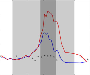
Figure 4 shows the evolution of  $\lambda _3$. We see that in all the FWO tests,
  $\lambda _3$ remains approximately zero throughout the flume, as expected in a Gaussian sea state. In both UWO and UWC tests, cases 4–9 show evident local increase of
  $\lambda _3$, indicating the manifestation of NED over the bar crest. We notice that the following current further enhances the maximum value of
  $\lambda _3$ (see the red curves), and extends the region where
  $\lambda _3$ is enhanced. Besides, the spatial extent of the non-equilibrium area in the UWC tests increases for longer waves. In other words, a following current increases both the magnitude and the range of NED.

Figure 4. Evolution of skewness  $\lambda _3$ in (a–i) cases 1–9 for FWO, UWO and UWC set-ups, with the bar profile indicated by grey areas.
The evolution of  $\lambda _4$ is shown in figure 5. The same trends as for
  $\lambda _3$ apply for
  $\lambda _4$. It is observed that in cases 3 and 4, the values of
  $\lambda _4$ get locally enhanced over the bar with the following current, whereas no such increase is noticeable in the corresponding UWO tests. For cases 5–9, the NEP is stronger in magnitude and lasts longer in space in the UWC scenario, in comparison with the UWO tests. Taking case 8 as an example, the maximum value of
  $\lambda _4$ is increased from 4.3 in the UWO set-up up to 5.0 in the UWC set-up. This would imply a heavier tail in the wave height distribution, and therefore a higher freak wave probability.

Figure 5. Evolution of kurtosis  $\lambda _4$ in (a–i) cases 1–9 for FWO, UWO and UWC set-ups, with the bar profile indicated by grey areas.
It should be noticed that the MI is not responsible for the local increase of  $\lambda _3$ and
  $\lambda _4$ in this study. For the UWC tests, in the upstream flat area with
  $h_1=1$ m and
  $U_1=0.1\,{\rm m}\,{\rm s}^{-1}$, the MI is expected to manifest for
  $k_ph_1 > 1.39$; over the bar crest with
  $h_2=0.4$ m and
  $U_2=0.25\,{\rm m}\,{\rm s}^{-1}$, the threshold for MI increases to
  $k_ph_2 > 1.48$ (see equation (41) in Liao et al. (Reference Liao, Dong, Ma and Gao2017)). For the UWO tests, the
  $k_p h$ threshold for MI is always
  $1.36$. Therefore, waves in all cases are modulationally stable over the bar crest.
Undoubtedly, the UWC set-up considered in this study is complicated, involving wave–wave, wave–bottom, wave–current and current–bottom interactions. Based on the analysis of the threshold water depth with current effect taken into account, the MI is considered to be insignificant for the local increase of skewness and kurtosis over the bar crest. The uneven bottom could increase the vorticity of the fluid, but this could be omitted considering the gentleness of the slope.
The uneven bottom might also give rise to free-surface deformation when a pure (steady) current passes over, as a result of significant current–bottom interaction (e.g. Buttle et al. Reference Buttle, Pethiyagoda, Moroney and McCue2018; Akselsen & Ellingsen Reference Akselsen and Ellingsen2019). It should be pointed out that such current-induced free-surface deformation (CIFSD) is a steady solution, i.e. the CIFSD is time-independent when the steady state is achieved. The CIFSD can therefore be considered as a change of the local mean water level, resulting in a change of the local water depth. The wave evolution may therefore be influenced by the CIFSD. In the present study, the current was generated 10 min before the wave-paddle started to move, so the steady state of the flow field was achieved, and the steady profile of the CIFSD over the bar crest was well established. Following equation (2.4) in Buttle et al. (Reference Buttle, Pethiyagoda, Moroney and McCue2018), the maximum magnitude of CIFSD is approximately 0.003 m for our experimental tests. As it represents a very small variation of the water depth over the bar crest ( $0.003/h_2 < 1\,\%$), we consider that the contribution of CIFSD to the evolution of central moments like skewness and kurtosis is minor and can be safely neglected in our study. In all, it is considered that the presence of the uneven bottom gradually changes the mean horizontal flow velocity without changing the (near) uniformity of the horizontal flow velocity along the
  $z$ axis, and that the occurrence of CIFSD does not contribute to the local changes of
  $\lambda _3$ and
  $\lambda _4$ over the bar.
We understand that the accelerating following current enhances and extends the local increase of  $\lambda _3$ and
  $\lambda _4$ as follows. A following current affects the surface waves in two aspects: on the one hand, it decreases the significant wave height (conservation of wave action); on the other hand, it decreases the wavenumber (Doppler effect). Both the steepness
  $\epsilon$ and the relative water depth
  $\mu$ are therefore decreased. The relative water depth over the shallower region
  $k_ph_2$ plays a dominant role in the manifestation of NED, smaller
  $k_ph_2$ resulting in stronger NEP. Thus, it is understandable to observe higher levels of
  $\lambda _3$ and
  $\lambda _4$. Compared with the UWO tests, the following current in the UWC tests increases the level of medium inhomogeneity and a longer spatial distance is needed for the sea state to adapt to the new equilibrium state.
3.2. Saturation depth for the maximum values of skewness and kurtosis
Figure 6 further illustrates the relationship between the maximum values of  $\lambda _3$,
  $\lambda _4$ (representing the magnitude of the NED) and the relative water depth
  $k_ph_2$ over the bar crest. The blue curve represents all 11 cases under the UWO condition and the red curve cases 1–9 under the UWC condition. Values of
  $k_p$ are computed with the current velocity taken into account (using (2.3)). It is shown that the evolution trends of maximum values of
  $\lambda _3$ and
  $\lambda _4$ as functions of
  $k_ph_2$ are very similar in UWO and UWC scenarios (given
  $k_p$ computed with proper dispersion relation). In our experiments, the NEP starts to appear for
  $k_ph_2 \approx 0.8$ (the above-mentioned ‘transition’ depth).

Figure 6. Maximum values of skewness (a) and kurtosis (b) over the shallower region as a function of the relative water depth over the bar crest.
Furthermore, figure 6 shows that the increase of  $\lambda _3$ and
  $\lambda _4$ with the decrease of
  $k_ph_2$ seems to stop for
  $k_ph_2 \approx 0.45$. This is not surprising since the increasing trend of
  $\lambda _3$ and
  $\lambda _4$ cannot be sustained unlimitedly. We refer to this particular relative water depth
  $k_ph_2 \approx 0.45$ as the ‘saturation depth’ of the NED. Below that saturation depth,
  $\lambda _3$ and
  $\lambda _4$ will no longer increase with a decrease of
  $k_ph_2$. As the peak period
  $T_p$ increases, the relative water depth decreases throughout the flume. The difference between the shallower and the deeper depth (i.e. the change of condition) also reduces; therefore, the non-equilibrium responses are weakened and the increasing trends of
  $\lambda _3$ and
  $\lambda _4$ slow down as well.
The saturation depth has been indicated (without defining a terminology) in the theoretical work of Mendes et al. (Reference Mendes, Scotti, Brunetti and Kasparian2022), where those authors consider the enhancement of  $\lambda _3$ and
  $\lambda _4$ takes place for
  $k_ph_2 \in [0.5, 1.5]$. Yet, such a saturation depth has never been reported in experimental works. It is anticipated that as the water depth decreases further, the wave evolution would be dominated by other effects, such as shallow-water effect and depth-induced breaking effect. Investigating these effects is certainly of academic and practical significance, yet it is beyond the present discussion of NED.
To further illustrate the ‘saturation’ effects, figure 7 superimposes the evolution of  $\lambda _3$ and
  $\lambda _4$ in four cases: cases 8 and 9 in the UWC scenario and cases 10 and 11 in the UWO scenario. In all these cases,
  $k_ph_2$ is considered saturated. It can be observed that the spatial profiles of
  $\lambda _3$ and
  $\lambda _4$ are very similar in these cases. Especially, the evolution of
  $\lambda _3$ is almost identical. When
  $k_ph_2$ saturates, in addition to similar maximum values of
  $\lambda _3$ and
  $\lambda _4$, we also notice that the following current does not result in a longer spatial range of NED. As a cross-validation for the saturation depth, we add in figure 7 one of the experimental results of Zhang et al. (Reference Zhang, Benoit, Kimmoun, Chabchoub and Hsu2019), obtained in a wave flume of Tainan Hydraulics Laboratory (THL). In the THL experiments, the bathymetry is composed of two flat regions connected by a constant upslope (
 $1/20$). Here, we only take case 3 reported in Zhang et al. (Reference Zhang, Benoit, Kimmoun, Chabchoub and Hsu2019), in which
  $k_ph_2$ happens to be
  $0.45$ (
 $T_p=2.5$ s,
  $h_2=0.3$ m, no current). In figure 7, the evolution of
  $\lambda _3$ and
  $\lambda _4$ of THL case 3 of Zhang et al. (Reference Zhang, Benoit, Kimmoun, Chabchoub and Hsu2019) (black curves) is shifted in space, so that the positions of maximum
  $\lambda _3$ and
  $\lambda _4$ align with the present results. Despite considerably different configurations, the spatial profiles of
  $\lambda _3$ and
  $\lambda _4$ of THL case 3 are in good agreement with the present results. It should be understood that
  $\lambda _3$ keeps a high level after 30 m in THL case 3 because there is no de-shoaling process. Therefore, we speculate that the saturation depth
  $k_ph_2 \approx 0.5$ has some universal relevance, though this needs to be confirmed by additional investigations.

Figure 7. Evolution of skewness (a) and kurtosis (b) in cases 8–11, and in case 3 reported in Zhang et al. (Reference Zhang, Benoit, Kimmoun, Chabchoub and Hsu2019). In all cases,  $k_ph_2$ is below the saturation depth.
4. Conclusion
We experimentally investigated the NED of surface waves induced by medium inhomogeneity, here provoked by spatially varying water depth and current velocity. In this experimental campaign, 11 irregular wave conditions have been tested under FWO, UWO and UWC scenarios. The results show that a following current could amplify the medium inhomogeneity as waves propagate over a shoal, such that higher peaks and wider spatial extents of the local enhancement of skewness  $\lambda _3$ and kurtosis
  $\lambda _4$ are achieved. The probability of freak waves is therefore enhanced due to an accelerating following current. This is because the decrease of the relative water depth can overwhelm the decrease of wave steepness, resulting in stronger sea-state NED response over a larger spatial extent. The maximum values of
  $\lambda _3$ and
  $\lambda _4$ achieved over the bar crest increase with the decrease of
  $k_ph_2$ in the UWO tests, and the relationships hold for the UWC tests with
  $k_p$ evaluated with the current velocity taken into account.
The evolution of maximum  $\lambda _3$ and
  $\lambda _4$ as functions of
  $k_ph_2$ shows two particular thresholds of relative depth: one is the so-called ‘transition depth’ (Trulsen et al. Reference Trulsen, Raustøl, Jorde and Rye2020), below which the NED starts to manifest (approximately
  $0.8$ in our experimental set-up); the other one is approximately
  $0.45$–
 $0.5$, below which the maximum
  $\lambda _3$ and
  $\lambda _4$ no longer increase with a further decrease of
  $k_ph_2$, the latter being named ‘saturation depth’. To the best of our knowledge, this saturation depth has never been reported in previous experimental works.
The present results are of high practical importance, especially for the assessment of freak wave risks in coastal areas with ambient currents. We have demonstrated that, somewhat counter-intuitively, a following current entering a shallow-water area increases the risk of extreme waves in that area.
Acknowledgements
The authors are grateful to the three anonymous reviewers for their valuable suggestions on various aspects that have considerably improved the paper, in particular on the discussion of CIFSD.
Funding
This work was supported by the National Natural Science Foundation of China (grant nos. 52101301; 51720105010), the China Postdoctoral Science Foundation (grant no. 2021M690523) and the Innovative Research Foundation of Ship General Performance (grant no. 31422119).
Declaration of interests
The authors report no conflict of interest.


