Introduction
The momentum balance equations of continuum sea-ice drift models include an internal friction term for describing how internal ice dynamics affect the drift. This includes floe–floe interaction (e.g. colliding and shearing) and mechanical thickness increase (e.g. ridging). The internal friction is described in terms of an internal stress state, which is linked to ice drift and thickness through a rheological model, the most widely used being the viscous–plastic rheology of Reference HiblerHibler (1979). The rheology includes a parameter interpreted as the aggregate compressive strength of ice cover in scales much larger than the characteristic floe diameter. The value of the strength parameter is set by validation exercises and is of the order of 15–30 kPa (Reference Hibler and WalshHibler and Walsh, 1982; Reference Kreyscher, Harder and LemkeKreyscher and others, 1997).
On the other hand, a single pack-ice floe as a solid body has a physical stress state that is a combination of thermal stresses and dynamical stresses generated by atmospheric and oceanic forcing. The dynamic stresses are transmitted at floe contacts and can propagate over large distances in a compact ice cover. The propagation patterns are expected to reflect the complicated geometry of the pack ice, and the upper limit of stresses is set by the material strength of sea ice, which is of the order of 1 MPa (Reference Timco and WeeksTimco and Weeks, 2010). Thus there is a scale effect of two magnitudes between modeled aggregate strength and the material strength.
The relation of large- and local-scale stresses is not yet well understood. There are two aspects to this problem. One is describing stress propagation and the role of the scale effect. The second is a fundamental question on the physical basis of continuum rheologies of ice models, especially as the viscous–plastic approach does not include elastic stresses central to the stress propagation. To address these issues, several campaigns have deployed stressmeter arrays on ice floes. Earlier campaigns used pressure-cell arrays (Reference Croasdale, Comfort, Frederking, Graham, Lewis, Sackinger and JeffriesCroasdale and others, 1988; Reference Coon, Lau, Bailey, Taylor, Axelsson and FranssonCoon and others, 1989), while many later Arctic campaigns (Reference Tucker and PerovichTucker and Perovich, 1992; Reference Richter-Menge and ElderRichter-Menge and Elder, 1998; Reference Richter-Menge, Elder, Claffey, Overland, Salo, Squire and LanghorneRichter-Menge and others, 2002a,Reference Richter-Menge, McNutt, Overland and Kwokb) used a biaxial stressmeter similar to that described by Reference Cox and JohnsonCox and Johnson (1983). Basic understanding of the variation of stressmeter records and their relationships with dynamic forcing has been attained, but bridging towards the large scale has advanced little as the arrays have not been extensive enough to really resolve the stress state of the floe. The stress propagation within a floe depends on the changing of floe–floe contacts and on thickness variation and other inhomogeneity within the floe. This shows in the stress records as spiky high-frequency variation and as spatial variation even over short horizontal or vertical distances.
This paper addresses the basic problem of comparability of stressmeter records, which is the prerequisite for inferences on the global stress state of an instrumented floe and beyond. It is not self-evident how ‘stress level’ should be defined for stress record comparisons such as ‘stress level for stressmeter 1 is k times that for stressmeter 2’. This is especially so if conclusions like ‘stress level at 10 m from the floe edge is k times that at 100 m from the edge’ follow. The stress peaks typically occur at different times at different locations and the comparison of instantaneous stress values is seldom informative. Thus ‘stress level’ is understood here to characterize a period with several stress peaks. Two obvious candidates for ‘stress level’ are then the stress record average over the period, which does not indicate much about the dynamically intensive events, and the highest stress peak, which has a singular character. It is shown that extreme value analysis can bridge between these two alternatives and provide simple and effective tools of stress level characterization.
The main objective of the present analyses is to develop means that can be used to make inferences on the spatial stress distributions present in a system of many floes from time domain stress records measured on a single floe. This is crucial for the development of ice models seeking to derive model physics from discrete subgridscale processes of floe systems. Spatial stress distributions are also needed to estimate the magnitude of local stresses driving the ridging process or exerting forces against ships and structures. Applicable theoretical tools may already be present in the granular media research (e.g. Reference Aranson and TsimringAranson and Tsimring, 2006) as it appears clear that pack ice is a granular medium, although one with extremely large variation in grain size and shape. The present paper seeks to point out one possible approach towards establishing a connection between granular media research and sea-ice research.
Data
Archived stress records from Sea Ice Mechanics Initiative (SIMI) Alaskan Beaufort Sea camp 1993–94 were reanalyzed. As described by Reference Richter-Menge and ElderRichter-Menge and Elder (1998), the mostly multi-year ice camp floe was 2–3 km in diameter and rather round, the average thickness was 1.4 m and the thickness range was 0.4–4.0 m. The floe contained a stripe of first-year level ice but no pronounced ridges. The initial location was ∼450km north of the Alaskan coast in the Beaufort Sea. The stress monitoring continued from October 1993 through March 1994 during which the floe drifted 250 km to the west from its initial location and rotated ∼60°. Biaxial vibrating wire stressmeters were installed at the center and edge of a floe. The triangular measurement configuration consisted of three edge sites and a floe center site. Seven sensors were placed on each edge site ∼0.25cm below the surface. The arrays originally extended 75 m from the edge, but edge site 2 was soon abandoned and edge site 3 was moved 400 m towards the center. At the floe center site, three sensors were installed at depths of 0.4, 1.0 and 2.0 m below surface; however, the deepest layer did not produce proper data.
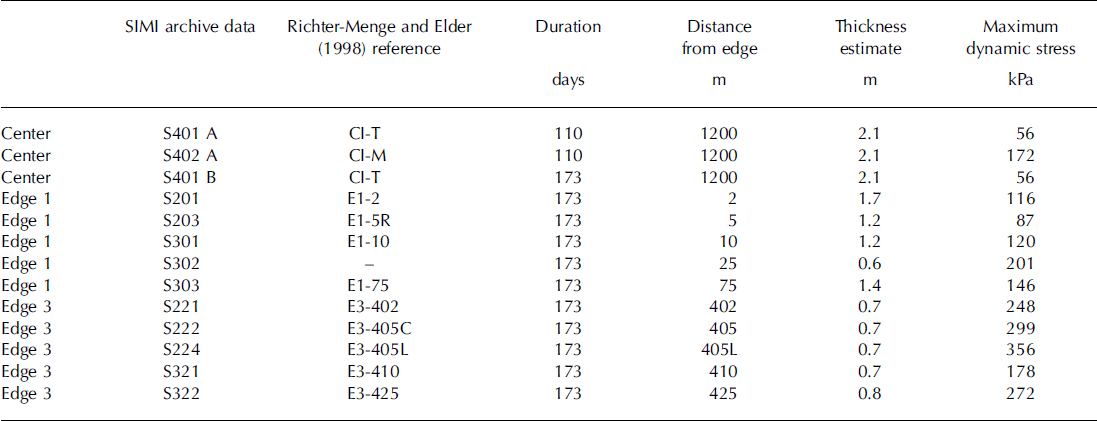
The details of the campaign are published in Reference Richter-Menge and ElderRichter-Menge and Elder (1998) and Reference Lewis and Richter-MengeLewis and Richter-Menge (1998). Great care was taken to calibrate the sensors and to determine the zero level before and after the experiment. In the final analysis the records from four sensors for edge site 1, five sensors for edge site 3 and two sensors at the floe center were considered reliable. The records of Reference Richter-Menge and ElderRichter-Menge and Elder (1998) are analyzed here with the addition of one archived record (Table 1).
Table 1. The analysed SIMI data. The 173 day range begins on 28 September and the 110 day range on 30 November 1993 and both end on 20 March 1994. The site names refer to the campaign of Reference Richter-Menge and ElderRichter-Menge and Elder (1998), which also included abandoned edge site 2
SIMI arrays used a biaxial stressmeter which allowed the determination of both principal components of the horizontal stress state. To obtain dynamic stresses, the contribution of thermally induced stresses must be separated. For reasons stated in Reference Richter-Menge and ElderRichter-Menge and Elder (1998) the standard procedure to obtain the dynamical stress estimate is to subtract the minor principal stress from the major principal stress. The stress record {xi} obtained thereby can be assumed to contain some error from the residual thermal stresses, zero level error and other sources,
All other sensors except the deeper center sensor share a common 173 day period that is used in most comparisons. A composite of all 173 day dynamic stress records of Table 1 is presented in Figure 1.

Fig. 1. Combined stress record, composed by selecting for each hour the maximum value from all eleven 173 day records.
Methods
In extreme value analysis the basic quantity is maximum stress value during a period T. In the analysis the stress record is divided into time windows of duration T, and from each time window the maximum value × is selected. These maxima have distribution fT
(x), which is an extreme value distribution, and their average is xT. The duration of the time window can be varied between sampling interval T
min and the stress record duration T
max. The sampling interval defines the average stress value
![]() for the stress record, and the record maximum stress value is
for the stress record, and the record maximum stress value is
![]() . Scaling properties pertaining to the extreme value distributions are relations between fT(x) and fλT(x), where A is a scaling factor. The scaling is statistically self-affine when
. Scaling properties pertaining to the extreme value distributions are relations between fT(x) and fλT(x), where A is a scaling factor. The scaling is statistically self-affine when
where H is the Hurst exponent (after Reference Hurst, Black and SimaikaHurst and others, 1965). Self-affine scaling generalizes the self-similar scaling of fractal curves so that it can be applied to time series (Reference FederFeder, 1988). As time and stress are different physical quantities they cannot be assumed to scale with the same ratio. Instead, different scaling factors are used and in the self-affine case of Eqn (2) these are T→ λT and x→ λ
H
x. Roughly, if this scaling is applied to the time series it will ‘look the same’ as the unscaled time series. If Eqn (2) applies then fT(x) is a Gumbel type II (Frechet) extreme value distribution, which is one of three possible asymptotical extreme value distributions (Reference Ang and TangAng and Tang, 1984). This can be seen by considering the cumulative distribution FT
(x) and λ = n. For a longer nT period, using the basic multiplication formula
![]() of extreme value statistics,
of extreme value statistics,
This functional equation is readily solved by taking logarithms, and the resulting Gumbel type II distribution is

Here Γ is the gamma function. Differentiation gives fT (x), but as FT(x) is the probability that the stress does not exceed × it is often more applicable in practical contexts. It is usually expressed as return period T/(1–FT ) or the expected interval between two exceedances of stress level x.
The method to check the potential self-affinity and to determine the distribution parameters is as follows. The time window duration T is varied over range, and a range of averages xτ is calculated. When the pairs (T, xT ) are plotted in a double logarithmic scale, the valid range for the self-affine relationship
appears as a straight line with slope H. Here T0 is a reference period selected from the valid range. This relationship, or (T, xT) plot, is the main tool of data comparison here. The SIMI data sampling interval Tm in is 1 hour and the binary range
was used. The diurnal range of {1,3,6,12,24} hours thus continues as a monthly range of {1,2,4,8,16,32} days. The general features of the SIMI (T, xT) plots are illustrated in Figure 2. The error term in Eqn (1) raises the values xT for shorter time windows. For longer windows the dynamic stress peaks and the self-affine statistics of dynamic stresses begin to dominate, typically when T exceeds 1 day. For T>32 days the number of time windows is too small for calculating the average xT. Thus the range 1–32 days is used throughout to determine H, and the reference period is selected to T 0=1 day. From Eqn (1) it can further be hypothesized that the observed value x 1hour , or the time-averaged dynamic stress, is an overestimate and a better estimate is obtained by extrapolating the linear slope down to 1 hour. The extrapolation of the slope to stress record duration Tmax, in most cases 173 days, provides an estimate for expected maximum stress instead of the observed singular value which is a random sample from FTmax(x). The extrapolation can be continued to longer periods (e.g. 1 year).
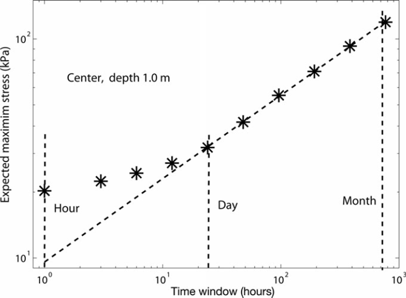
Fig. 2. The expected maximum stress xT as a function of time window T for center site stressmeter S402 A. The stress record duration is 110 days and T ranges from 1 hour to 32 days. The power-law dependence for windows longer than 1 day and the deviation upwards from the power law for shorter windows are typical features. The extension of the power-law slope downwards gives an average dynamic stress estimate about half of the observed value.
Results
Center site
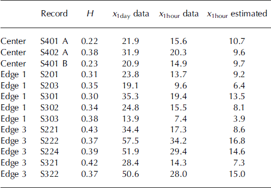
The center site had stressmeters S401 and S402 at 0.4 and 1.0 m below the surface in 2.1 m thick ice. Their common 110 day period starts from the deployment of the deeper stressmeter on 30 November 1993 and is chosen to end on 20 March 1994, which is the last day for edge site records in Table 1. The (T, xT ) plots of Figure 3 are in agreement with self-affinity and show large differences between the stress levels and exponents. The exponents for the slopes are 0.22 and 0.38 and the reference values x 1day are 22 and 32 kPa for 0.4 and 1.0 m depth, respectively. On the other hand, the observed values x 1hour are close to each other (Table 2) and the same applies to the values of 11 and 10 kPa obtained by extrapolating the slopes in Figure 3 to 1 hour. Remarkably the upper stressmeter results are very similar both for the 110day record and for the 173 day record used when comparing this stressmeter with edge sites.
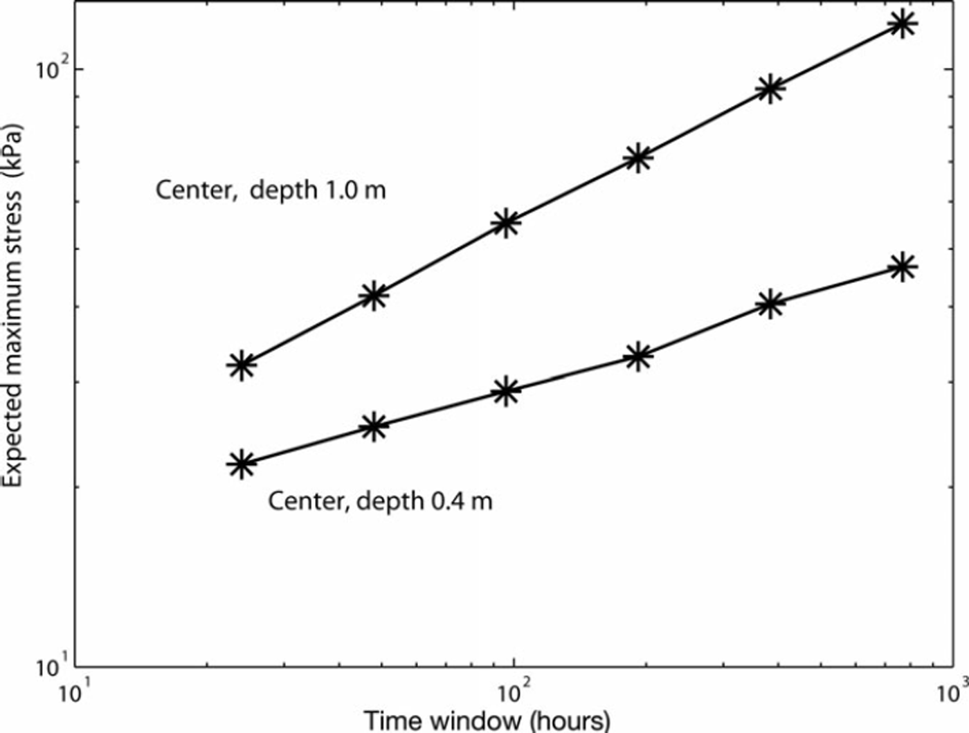
Fig. 3. Expected maximum stress xT as a function of time window T for the two center site stressmeters deployed at the same location at different depths. The stressmeter record duration was 110 days, and the time window ranges from 1 to 32 days.
Table 2. Self-affine parameters for the analyzed profiles
Edge site 1
The site name refers to that in Reference Richter-Menge and ElderRichter-Menge and Elder (1998). The five stressmeters, with locations ranging from 2 to 75 m from the edge, were deployed at depths between 0.20 and 0.44 m. The site contained both first- and multi-year ice, and thickness variation was large, 0.6–1.7 m at the stressmeter locations. The exponent from linear fit varies between 0.30 and 0.38, with a mean of 0.34, but the order of profiles for x 1day is the same as for x 32days except for the pair 2 and 25 m from the edge (Fig. 4). The general appearance is that the (T , xT) plots describe more or less similar self-affine loading processes where only the stress level varies significantly while H remains about the same. The ratio of highest and lowest stress level is about 2.5, but no clear dependence between stress level and distance from the edge can be found.
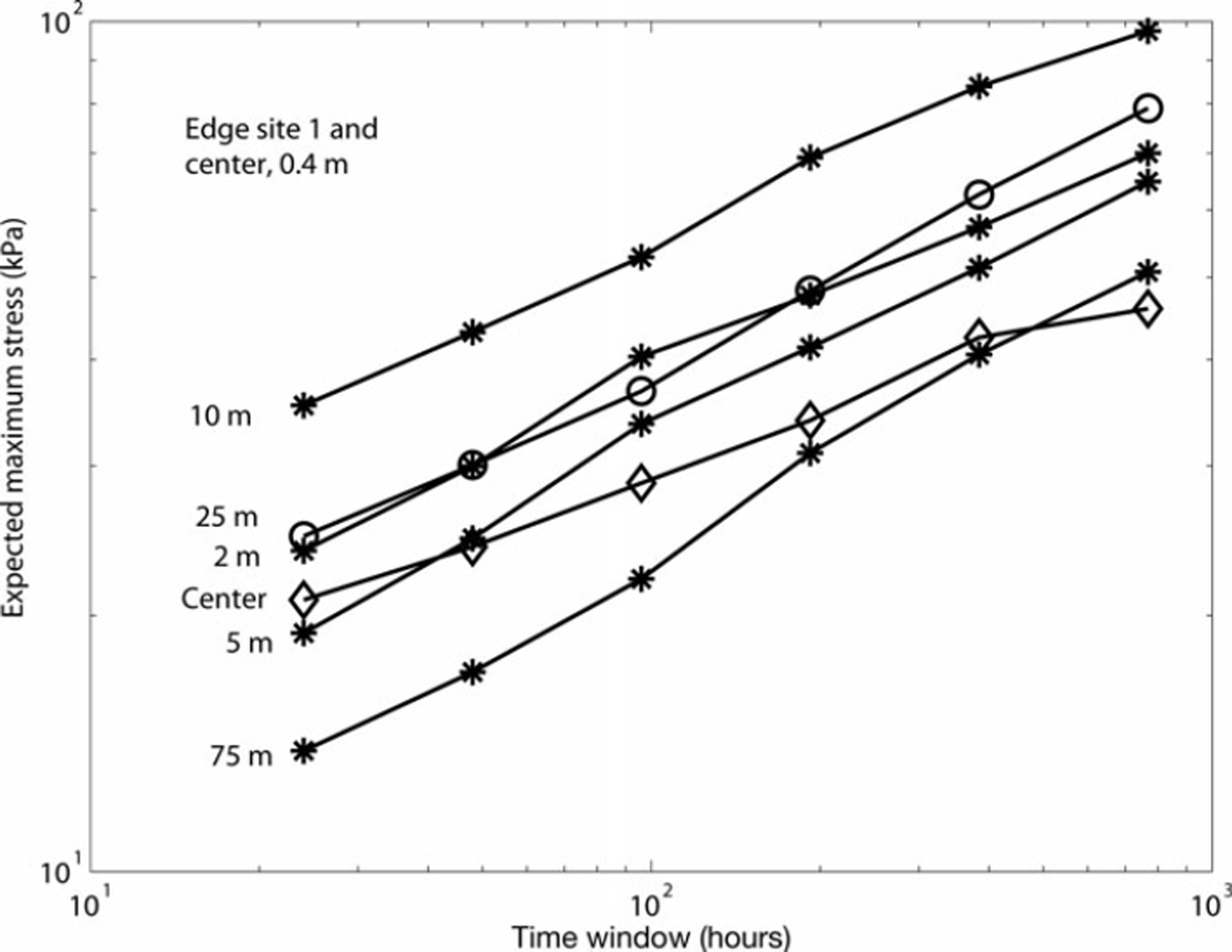
Fig. 4. Expected maximum stress xT as a function of time window T for edge site 1 containing five stressmeters at different distances from the ice edge. The upper center site sensor is included for comparison. The stressmeter record duration was 173 days and the time window ranges from 1 to 32 days.
Edge site 3
The site name refers to that in Reference Richter-Menge and ElderRichter-Menge and Elder (1998). The five stressmeters were located within 25 m at a site that was ∼400m from the floe edge. The variation in deployment depth ranged from 0.20 to 0.26 m and the ice thickness at the stressmeter locations from 0.7 to 0.8 m. The variation in both deployment depth and thickness is much less than at edge site 1. The slopes of (T , xT) plots in Figure 5 are very similar and the exponent H varies little around the mean value 0.40. The stress levels are higher on average than at edge site 1. The self-affine characteristics are almost identical for all profiles, but the stress level varies significantly, the ratio of highest and lowest stress level being ∼2. This runs counter to the expectations raised by the uniformity of the ice and deployment conditions.
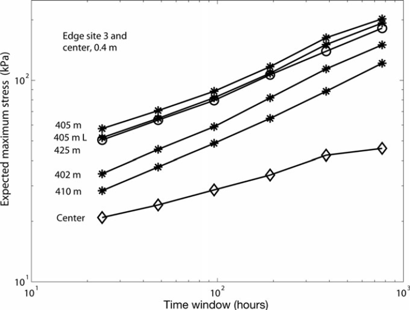
Fig. 5. Expected maximum stress xT as a function of time window T for edge site 3 containing five stressmeters in a close arrangement 400–425m from the floe edge. The upper center site sensor is included for comparison. The stressmeter record duration was 173 days, and the time window ranges from 1 to 32 days.
Combined records and seasonal variation
Combined records that can be used to characterize the floe stress state were calculated from the eleven 173 day records in two ways. First, an average record was calculated. The other, a maximum composite record, is constructed by selecting for each time instant the highest observed stress value (Fig. 1). Both composites produced almost perfect linear slopes in the logarithmic (T, xT ) plot and had the same exponent H = 0.34. The three stress level parameters in Table 3 are 2.2 times higher for the maximum composite. To the two composite records pertains also a third one, the record of spatial variation. This was obtained by calculating the standard deviation for each time instant and found to be self-affine with H=036. Moreover, these three records are strongly correlated, with r≥0.94 in all cases, and in linear regression the floe maximum is 2.2 times the mean value and 3.5 times the standard deviation. Thus the spatial variation is at most weakly dependent on stress level.
Table 3. Combined records and seasonal comparisons for the maximum composite
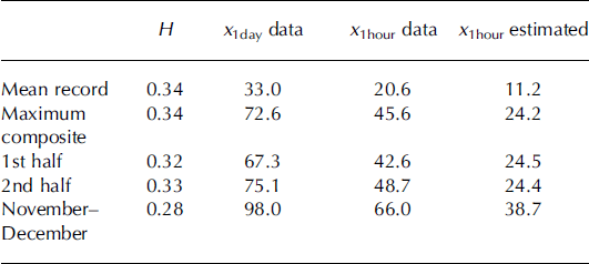
The seasonal variation was studied from the maximum composite record for three periods (Table 3). The record was first divided into two halves, the day of demarcation being 24 December. The two halves have about the same parameters H and estimated x 1hour as the whole profile, so the seasonal variation if it exists is not dominating. The third period is from 1 November to the end of December. During this period the dynamic activity in the ice cover had more intense and persistent characteristics and the stress level remained >50kPa for weeks. The analyses by Reference Lewis and Richter-MengeLewis and Richter-Menge (1998) pertain to the last 25 days of this period. Lower exponent and higher reference stress levels are observed.
Baltic Sea comparison
A short comparison is made with Baltic Sea data. The record of Figure 6 is from the southern Bay of Bothnia and was measured between 27 February and 11 March 2011 with a biaxial stressmeter similar to the SIMI records. The level ice thicknesses in the deformed ice cover were ∼0.6m. The wind speed exceeded 10 ms–1 most of the time, and there was intermittent ice drift to the northeast. The stress peaks are related to phases of ice drift, except the highest one which is associated with stress build-up during a static period before the next drift onset. Similarly to SIMI data the logarithmic (T, xT) plot assumes linearity after x 1day. The parameters determined from the range of [1,2,4] days are H=0.52, x 1day = 27.0 kPa and measured/estimated x 1hour of 9.2 and 5.1 kPa, respectively. The stress levels are lower, but the exponent is higher, which probably reflects the intermittent stick-slip motion of the coastal ice field although solid conclusions are not warranted due to the shortness of the record. However, as an interesting detail the parameters predict 1 year maximum stress of 572 kPa, close to the corresponding SIMI prediction.

Fig. 6. (a) A 2 week stress record from the Baltic Sea and (b) the associated dependence of expected maximum stress xT on time window duration. The time window ranges from 1 hour to 4 days.
Discussion
The exponent H and stress distributions
The studied stress records show clear self-affine characteristics. A self-affine record can be described by Hurst’s exponent H and some reference stress, here x 1day. The exponent was determined from average maxima ranging from 1 day to ∼1 month and it tells that if the time period is doubled, the expected maximum stress increases by 2H. It is in general a measure of the inhomogeneity or clustering of the stress peaks. For higher H, the peaks are more concentrated in certain periods; for low H they are more regularly recurring and the process more stationary. It can be hypothesized that the stress records would become more stationary for very long Tas the maximum values are limited by the material strength of ice. The slope of the (T, xT) plot would then turn gradually horizontal. However, there are no indications of this in the 6 month records.
The exponent can often be determined from (T, xT) plots also when the Gumbel II distribution is not a very good model for observed fT (x). For the present data the Gumbel II fits the tail part of the distributions but not well around the mode. However, the Gumbel II has only asymptotical validity. The low stress values also contain thermal signals, which are not expected to be of Gumbel II type. The poor fit may also be related to the ambiguity of zero level, especially as the histogram for low values of × is often irregularly multimodal, possibly also due to instrument zero drift. For large × these problems have less effect and the Gumbel II can be used for return period estimates. As such this result has applications, especially as relates to the loading state at the floe edge. For example, estimates can be made of the compressive loads suffered by a ship between two floes.
The stress level and its dependence on location
The reference stress level, 1 day average maximum x 1day, ranges from 13.9 to 57.5 kPa and the mean value of the records (31.9kPa) is close to the value for the averaged record (33 kPa). The estimated average dynamic stress x 1hour ranges from 3.9 to 16.8kPa. The possible factors contributing to this variation are the distance from the floe edge, deployment depth, the location in relation to the stress-transmitting edge contacts, and thickness variation.
There is no clear pattern in the stress levels in relation to the distance from the floe edge. The SIMI floe with average thickness 1.4 m was composed of multi- and first-year ice with characteristic thicknesses of 2.0 and 0.5 m, respectively. Thus stresses propagating across the floe would show four times higher vertically averaged values in the thinner ice type. In principle the line load per horizontal length unit (kN m−1), or stress multiplied by thickness, should then be better suited for spatial variation considerations.
However, no clear dependency of line loads on the distance from floe edge was found between the sites or within them. Edge site 1 had much thickness variation with multi- and first-year ice and some shallow ridge keels. On the other hand, the edge site 3 stressmeters at 402–425 m from the edge are, relative to floe radius, more or less at the same spot and the thickness variation is small. Still the variation of line loads is not much different from site 1. Considering 1 day maximum line loads, the values 29 and 13 kNm−1 are found for the array average and standard deviation at edge site 1, while the same values for edge site 3 are 32 and 10 kNm−1. Thus from the line load viewpoint the characteristics of the two sites appear rather similar. At the center the line loads are somewhat higher, but it is likely that multiple locations would have shown similar variation to that in edge site 3. On the other hand, the vertical variation observed at the center may also have been present at other sites. The conclusion is more or less that the long-term stress state is about the same at all locations on the floe and could be determined with a local array of a sufficient number of stressmeters deployed at different depths. The origin of the stress level variation remains unclear, but edge site 3 results, in particular, indicate that the variation is a persistent feature.
The stress state of the floe
The exponent H ranges from 0.22 to 0.43, and the mean value of 0.35 is almost equal to the value, 0.34, of the combined records. The value 0.34 characterizes more the overall response of the SIMI camp floe to the loading imposed along its edge by contacting neighbor floes, while the local values depend in addition on the stress propagation within the floe. Little is known about how stresses propagate in a floe system and the scale over which the far field stresses and events are felt by the stressmeters. The SIMI floe did not deform much, but the typical spiky character of the stress records is indicative of remote deformation events where local stress is first built up and then relieved. As the floe drifted and rotated, the edge contact geometry must have been changing. This is also indicated by the location of the maximum stress value for each hour, as this changed period-wise from one array to another and back. However, the two 3 month half-periods of the combined record have the same parameters as the whole period. This suggests that the periods are long enough to average out the effect of the changing edge contacts and that 0.34 characterizes the loading process and the surrounding ice cover in general. The period November–December gives somewhat different results, as is expected from Figure 1. There is clear sustained background stress level superposed by recurring stress peaks. The midwinter ice cover apparently has a more massive-like character with continuous quasi-stationary stress state. This is also indicated by the lower exponent (0.28) for this period.
Another dimension to the problem is the spatial variation observed between and within the arrays. It is not known how well either of the combined records represents the global floe stress state, especially as the planned rosette of identical edge sites could not be realized and the vertical variation is not known. However, it is likely, whatever the reference level, that the 1 hour global floe stresses make a self-affine record with H close to 0.34 as this value was shown to characterize the pack regionally.
Relation to ice kinematics
A major motivation for stress campaigns has been to reveal the relationship between ice stresses and ice kinematics and gain insight into how ice-drift model rheologies should be formulated. For the present data the relationship was studied by Reference Lewis and Richter-MengeLewis and Richter-Menge (1998). Although the larger-scale average stress is certainly related to kinematic states (e.g. rates of divergence, shear and total deformation), the stress record time variation is likely to be dominated by the stress propagation patterns that change with the changing floe-floe contacts. Therefore, only the statistical aspects of the kinematics-stress relationship are considered here. As contacting and detaching of floes involves local differential movements, the variation in the velocity field is used here as the kinematic counterpart of the stress variation.
The SIMI camp had 13 drifters, one at the central floe and the others in two roughly circular arrangements with radii ∼5 and ∼10 km from the central floe. The velocity time histories for the same 173 day period as in Figure 1 and Table 3 were studied and for each hour the standard deviation of velocity magnitude was calculated. This time series was analyzed similarly to the stress records and was found to show self-affine characteristics with exponent H=0.33 (Fig. 7). That this value is similar to those shown in Table 3 is a strong indication that the exponent characterizes the geometry of the regional floe system, which is then mirrored in the variation of drift velocity and stress.
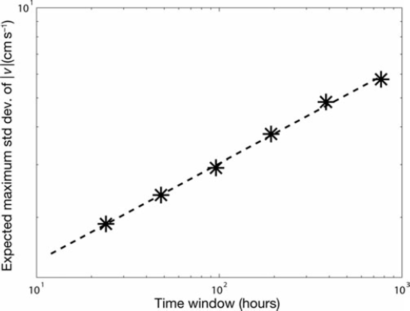
Fig. 7. Expected maximum for the standard deviation of the velocity magnitude as a function of the time window. Combined data from 13 drifters at and around the main floe are used.
The stress state of the pack
A single floe, even one for which the stress state is perfectly understood, is still not sufficient to characterize the ice pack. Granular materials research has demonstrated the large stress variation in stressed granular systems. The stresses are concentrated in a subsystem of branching chains between which there are stress-free lacunas, a phenomenon that has been well studied both experimentally and theoretically, although for systems much simpler than deforming pack ice (e.g. Reference Majmudar and BehringerMajmudar and Behringer, 2005). In any case, the intermittent spatial distribution of stresses has a time domain adjoint in the spiky stress records. A homogeneous isotropic system, consisting of identical floes and undergoing stationary deformation, is expected to show ergodicity. This means that the long-term time-averaged stress state of a floe equals the spatial average sampled at a single time instant from a large number of floes. Also, the distribution of stress values (e.g. at the floe center) would be the same when determined either way.
Thus if H characterizes the floe system regionally a simple starting assumption is that it pertains to spatial variation as well. The spatial distribution of floe stresses would then be self-affine with exponent H. It may be hypothesized further that the mean of this regional distribution is about the same as the internal stress of an ice model describing the pack and about the same as the long-term average of the SIMI floe, or ∼10–20kPa. Then in a regional linear array (gridcell boundary) with a scale of 30 characteristic floe diameters the expected maximum floe stress is 30 H times or about three times the regional average (H=0.34), and in a region (gridcell) of 30 × 30 characteristic floe diameters is ten times the regional average. These are in agreement with the present understanding of the ice strength scale effect (Reference DempseyDempsey, 2000).
Conclusions
Geophysical time series with several sources of randomness can be hard to analyze as the connection to the basic dynamic processes behind the observed variation lies hidden. For ice stress the randomness comes from the complicated floe geometry and thickness variation and, on the other hand, from the constantly changing patterns of stress propagation over chains of contacting floes. Extreme value methods can often provide the first stronghold in the analysis. They were used here to separate the effect of the loading process, occurring along the floe boundary, and the stress level, which also depends on floe geometry and other more contingent features. This provided a stress record intercomparison method, characterizations of the global stress state of the floe, a connection to kinematic statistics and a possible scaling for stress distributions in a floe system. The results also give new insights for studies on the relationship between continuum rheologies and subgrid-scale discontinuous processes, for example by Reference HiblerHibler (1977) and more recently by Reference Weiss, Schulson and SternWeiss and others (2007), and on the scaling exponents of the kinematic deformation fields (e.g. Reference Hutchings, Roberts, Geiger and Richter-MengeHutchings and others, 2011).
Acknowledgements
This research was conducted within the European Union-funded projects ‘Safety of winter navigation in dynamic ice’ (contract SCP8-GA-2009-233884-SAFEWIN). The partners in this project are Aalto University, the Arctic and Antarctic Research Institute, the Finnish Meteorological Institute, the Finnish Transport Agency, ILS Oy, Stena Rederi AB, the Swedish Maritime Administration, the Swedish Meteorological and Hydrological Institute, Tallinn University of Technology and the AS Tallink Group. The open access to US Army Cold Regions Research and Engineering Laboratory (CRREL) stress data is greatly appreciated.


