


1. Introduction
The Kelvin–Helmholtz instability (KHI) commonly occurs when there is velocity shear in a single continuous fluid or a velocity difference across the interface between two fluids. It leads to the progressive steepening of fluid interfaces and ultimately forms roll-up-like patterns in the flow (Gallaire & Brun Reference Gallaire and Brun2017). This makes KHI crucial in fluid mixing and transport processes, which are observed frequently in astrophysics (Roediger et al. Reference Roediger, Kraft, Nulsen, Churazov, Forman, Brüggen and Kokotanekova2013), river plumes (Horner-Devine, Hetland & MacDonald Reference Horner-Devine, Hetland and MacDonald2015), food processing, and medical and cleaning industries (Regner et al. Reference Regner, Henningsson, Wiklund, Östergren and Trägårdh2007; Landel & Wilson Reference Landel and Wilson2021; Jayaprakash et al. Reference Jayaprakash, Costalonga, Dhulipala and Varanasi2020). It is well-known that a shear flow with a streamwise velocity profile  $U$ that exhibits an inflection point (IP) where
  $U^{\prime \prime }=0$, becomes unstable according to the Rayleigh inviscid stability theory (Rayleigh Reference Rayleigh1879). This condition can trigger KHI by exacerbating the disturbances (Winant & Browand Reference Winant and Browand1974; Nepf Reference Nepf2012; Caulfield Reference Caulfield2021). A stratified layer arises when two fluids with different viscosities flow in the same or opposite directions in a miscible flow configuration. This may result in a velocity profile with an IP, which in turn can lead to the formation of KHI.
By conducting a linear stability analysis on parallel shear flow in a channel, Govindarajan, L'vov & Procaccia (Reference Govindarajan, L'vov and Procaccia2001) and Govindarajan (Reference Govindarajan2004) showed that the flow becomes unstable when the critical layer, or the wall-normal location where the phase speed of the disturbance equals the mean velocity, overlaps the viscosity-stratified layer. Under this condition, maximum disturbance kinetic energy is produced, which makes the flow unstable. It was shown that a slight viscosity stratification in the absence of reaction causes huge stabilization/destabilization by the KHI and some other instabilities in the Navier–Stokes-driven flow (Govindarajan & Sahu Reference Govindarajan and Sahu2014). However, the study on the effects of chemical reactions on viscosity stratification is nearly unexplored. A chemical reaction of  $A+B \rightarrow C$ type, where separate solutions of chemicals
  $A$ and
  $B$ undergo a reaction to produce
  $C$, is known to actively modify or control the convection of Darcy's flow by altering the viscosity profile. For instance, Podgorski et al. (Reference Podgorski, Sostarecz, Zorman and Belmonte2007) experimented with aqueous solutions of the cationic surfactant cetyltrimethylammonium bromide (CTAB) and the organic salt sodium salicylate (NaSal). It was found that bringing CTAB and NaSal into contact produces a strongly viscoelastic micellar material. The micellar gel-like medium was formed due to reaction–diffusion at the interface between two otherwise ordinary, miscible water-like Newtonian fluids of identical viscosities. The experiments were carried out in a Hele-Shaw cell, where new patterns forming fingering instability were observed. The experiment by Nagatsu et al. (Reference Nagatsu, Matsuda, Kato and Tada2007) justifies the concentration dependency of viscosity and its gradient increment or decrement by a chemical reaction of
  $A + B \rightarrow C$ type. They used the pH dependency of a viscous solution (aqueous polyacrylic acid, PAA) of polymers to tune the changes in the gradient of the mobility profile. Riolfo et al. (Reference Riolfo, Nagatsu, Iwata, Maes, Trevelyan and De Wit2012) claimed that the presence of NaOH induces viscous fingering because the neutralization reaction
  $\text {PAA} + \text {NaOH} \rightarrow \text {SPA}+ \text {H}_{2}\text {O}$ transforms the acid PAA into the more viscous salt sodium polyacrylate (SPA), and hence modifies the viscosity profile in the system. One can look at the theoretical studies too, where reaction induces instabilities by changing the viscosity profiles of the underlying fluids (Gérard & De Wit Reference Gérard and De Wit2009; Hejazi et al. Reference Hejazi, Trevelyan, Azaiez and De Wit2010; Sharma et al. Reference Sharma, Pramanik, Chen and Mishra2019; De Wit Reference De Wit2020). Thus it is natural to ask: can such a realistic chemical reaction of
  $A+B \rightarrow C$ type modify the viscosity at a very localized region so that an appropriate IP in the mean velocity profile generates the KHI? Moreover, it is necessary to investigate how the chemical reaction affects the stability of a layered flow in linear and nonlinear regimes.
In this context, the objective of this paper is to study the effects of viscosity stratification caused solely by a simple  $A+B \rightarrow C$ type chemical reaction in the Navier–Stokes flow. For this, we take two iso-viscous reactants
  $A$ and
  $B$ in a layered channel flow model that produce a product
  $C$ of different viscosity upon reacting with each other. We found that a favourable IP in the mean velocity for the KHI appears at one front of the reaction zone, depending on the viscosity of the reaction's product. In contrast, the other front influences the KHI negatively, causing it to diffuse steadily. The Kelvin–Helmholtz-type roll-up produces two distinct patterns due to this unusual reactive phenomenon. One of them is in good agreement with experimental results (Hu & Cubaud Reference Hu and Cubaud2018). Unlike previous approaches (Govindarajan & Sahu Reference Govindarajan and Sahu2014), we have used both linear stability analysis (LSA) and direct numerical simulations (DNS) to obtain stable and unstable zones in the parameter space spanned by the Damköhler number and critical log-mobility ratio. We demonstrate that the flow is more unstable when the product is less viscous through an asymmetric area occupancy of the instability region.
2. Mathematical formulation
Two concentrically flowing streams form downstream when a fluid displaces another fluid of different viscosity with a constant volumetric flow rate in a channel or pipe (Sahu et al. Reference Sahu, Ding, Valluri and Matar2009). Two interfaces separate the binary viscous fluids across the channel/pipe. Such a type of flow configuration is known as core-annular flow, and its features have been analysed extensively (Joseph et al. Reference Joseph, Bai, Chen and Renardy1997). However, the stability results (Selvam et al. Reference Selvam, Merk, Govindarajan and Meiburg2007; Talon & Meiburg Reference Talon and Meiburg2011) and unstable patterns (D'olce et al. Reference D'olce, Martin, Rakotomalala, Salin and Talon2009; Sahu et al. Reference Sahu, Ding, Valluri and Matar2009; Selvam et al. Reference Selvam, Talon, Lesshafft and Meiburg2009) are symmetric with respect to the centreline of the channel. So here we consider a two-layered flow configuration in a channel (see, figure 1a). One can extend this two-layered flow configuration to core-annular flow under symmetric boundary conditions at the middle height of the channel, and mimicking results can be expected from an appropriate scaling (Drazin & Reid Reference Drazin and Reid1985; Schmid & Henningson Reference Schmid and Henningson2001). Moreover, this configuration allows us to compare the experimental results of the non-reactive two-layered microfluidic flow (Hu & Cubaud Reference Hu and Cubaud2018). We choose a two-dimensional  $x\unicode{x2013}y$ plane channel of length
  $L$ and height
  $H$ for the DNS. Here, the two-layered configuration is constituted in the following way. A reactant fluid containing solute
  $A$ with dimensional concentration
  ${\mathcal {A}}$ of viscosity
  $\mu _{1}$ overlies another iso-viscous miscible reactant fluid containing solute
  $B$ with the same concentration
  ${\mathcal {A}}$ (see figure 1a). The initial stratification is along a horizontal flat interface located at
  $y=h$. Upon diffusive mixing across
  $y=h$, both solutions
  $A$ and
  $B$ react to produce
  $C$ of viscosity
  $\mu _2$ following simple bimolecular kinetics
  $A+B \rightarrow C$ (Gálfi & Rácz Reference Gálfi and Rácz1988). The reactants and the product fluids are assumed to be Newtonian and incompressible with equal density
  $\rho$. The chemical rate and the diffusion coefficients of solutes
  $A, B, C$ are assumed to be constant (Rongy, Trevelyan & De Wit Reference Rongy, Trevelyan and De Wit2008), i.e.
  $k$ and
  $D$, respectively. We use the reference length scale
  $H$, volumetric flow rate
  $Q$, concentration
  ${\mathcal {A}}$, viscosity
  $\mu _{1}$, velocity
  $Q/H$, time
  $H^{2}/Q$, and pressure
  $\rho Q^{2}/H^2$ to obtain the following coupled dimensionless Navier–Stokes equations with the reaction–diffusion–convection system:
 $$\begin{gather} \boldsymbol{\nabla} \boldsymbol{\cdot} \boldsymbol{u}=0, \end{gather}$$
 $$\begin{gather}\partial_{t} \boldsymbol{u}+\boldsymbol{u} \boldsymbol{\cdot} \boldsymbol{\nabla} \boldsymbol{u} ={-}\boldsymbol{\nabla} p+\frac{1}{R e}\,\boldsymbol{\nabla} \boldsymbol{\cdot}[\mu\left(\boldsymbol{\nabla} \boldsymbol{u}+\boldsymbol{\nabla} \boldsymbol{u}^{\rm T}\right)], \end{gather}$$
 $$\begin{gather}\partial_{t} A+\boldsymbol{u} \boldsymbol{\cdot} \boldsymbol{\nabla} A=\frac{1}{P e}\,\Delta A-D a \, A B, \end{gather}$$
 $$\begin{gather}\partial_{t} B+\boldsymbol{u} \boldsymbol{\cdot} \boldsymbol{\nabla} B=\frac{1}{P e}\,\Delta B-D a \, A B, \end{gather}$$
 $$\begin{gather}\partial_{t} C+\boldsymbol{u} \boldsymbol{\cdot} \boldsymbol{\nabla} C=\frac{1}{P e}\,\Delta C+D a \, A B, \end{gather}$$
 $$\begin{gather}\mu={\rm e}^ {(R_{c} C)}. \end{gather}$$
Here,  $\boldsymbol {u}=(u,v)$ is the velocity vector, wherein
  $u$ and
  $v$ are the axial and vertical components, respectively; and
  $p$ denotes the pressure. The viscosity is related to product concentration through (2.1f), which is an Arrhenius relationship. The above model system employs no-flux, no-slip and no-penetration conditions at the top and bottom walls. Periodic boundary conditions are used at the inlet and outlet of the channel. Four dimensionless numbers are associated with this problem. The Reynolds number
  $Re=\rho Q / \mu _1$, and the Péclet number
  $P e=Q/D$ signify the relative strength of convective to diffusive transport in the momentum and solutes, respectively. The Damköhler number
  $D a=(H)^{2} k {\mathcal {A}} / Q$ expresses the ratio between advection and reaction time scales, and the log-mobility ratio
  $R_{c} = \ln (\mu _{2}/\mu _{1})$. We aim to analyse the stability of the problem described by (2.1) in linear and nonlinear regimes. Thus below, we first calculate the base state solutions around which the growth of a tiny perturbation needs to be checked.

Figure 1. (a) The schematic of the problem. Base state profiles for (b) concentrations  $A,B,C$, (c) viscosity, (d) axial velocity, (e) zoomed second derivative of axial velocity near to the reactive zone, with various
  $R_{c}$ when
  $h=0.3$,
  $\delta =0.1$ (whose freezing time
  $t_{0}$ is
  $3.776$),
  $Da=100$ and
  $Pe=2 \times 10^{4}$.
2.1. Base-state concentrations, viscosity and velocity
Under the parallel flow assumptions, we assume the base-state concentrations  $A_{0}(y, t)$,
  $B_{0}(y, t)$ and
  $C_{0}(y, t)$ to be spatially varying only in the
  $y$-direction, while satisfying the following one-dimensional reaction–diffusion (RD) system of equations:
 $$\begin{gather} \partial_{t} A_{0} =\frac{1}{P e}\,\partial_{yy} A_{0}-D a \, A_{0} B_{0}, \end{gather}$$
 $$\begin{gather}\partial_{t} B_{0} =\frac{1}{P e}\,\partial_{yy} B_{0}-D a \, A_{0} B_{0}, \end{gather}$$
 $$\begin{gather}\partial_{t} C_{0} =\frac{1}{P e}\,\partial_{yy} C_{0}+D a \, A_{0} B_{0}. \end{gather}$$
Since the solution of  $A$ overlies the solution of
  $B$, and there is no product initially, the initial condition for the RD system is taken as
  $(A_{0}, B_{0}, C_{0})=(1,0,0)$ for
  $y > h$,
  $(A_{0}, B_{0}, C_{0})=(0,1,0)$ for
  $y < h$. The RD system does not have an analytical solution with this initial condition and no-flux boundary conditions. Moreover, the only possible solution is
  $A_{0}+B_{0}+2 C_{0}=1$, with the reaction front at
  $y=h$ (Gálfi & Rácz Reference Gálfi and Rácz1988). So we solve the RD system numerically on a uniform grid (with number of grid points
  $10^4$) by using the Crank–Nicolson method for underlying diffusion equations, while the reaction terms are handled explicitly.
At each time, the base-state viscosity is evaluated following the Arrhenius relation (2.1f), i.e.  $\bar {\mu }(y, t)=\exp ({R_{C} C_{0}(y, t)})$. By the quasi-steady-state approximation (Tan & Homsy Reference Tan and Homsy1987), the time variable is replaced with a constant time
  $t=t_{0}$, which is termed the freezing time. Thus the quasi-steady base-state concentrations and viscosity become functions of only
  $y$, and we denote them as
  $\bar {A}(y)$,
  $\bar {B}(y)$,
  $\bar {C}(y)$ and
  $\bar {\mu }(y)$, respectively. The mean flow profile
  $(u,v)=(\bar {U}(y),0)$ is obtained by solving the fully developed version of the Navier–Stokes equations,
  $Re\,(\mathrm {d} P / \mathrm {d}\kern0.7pt x )=(\mathrm {d}/\mathrm {d} y)(\bar {\mu }\,\mathrm {d} \bar {U}/\mathrm {d} y)$. An explicit expression of the exact analytical solution for
  $\bar {U}$ can be found in Talon & Meiburg (Reference Talon and Meiburg2011). Note that the pressure gradient
  ${\rm d}P/{{\rm d}\kern0.7pt x}$ is kept constant, assuming the non-dimensional flow rate
  $Q=\int _{0}^{1} \bar {U}\, {{\rm d}y} =1$.
Exemplary base state profiles of concentrations are shown in figure 1(b), which depicts clearly the formation of the product  $C$ of thickness
  $\delta =0.1$ around
  $h=0.3$. It is to be noted here that the freezing time
  $t_{0}=3.776$ leads to the formation of the product
  $C$ in layer width
  $0.1$. Figure 1(c) shows the base-state
  $C$ viscosity profiles for
  $R_{c}= -3$,
  $0$ and
  $+3$, depicting its variation across the height of the channel when the product's viscosity is less than, identical to and greater than the iso-viscous reactants, respectively. Figure 1(d) shows the
  $\bar {U}$ profile modified due to the viscosity variation arising from the chemical reaction. We observe that when
  $R_{c}=-3$, the velocity increases more than in the
  $R_{c}=0$ case in the upper layer (
 $y>h$), making the maximum velocity even greater than that of
  $R_{c}=0$ case. However, in the lower layer (
 $y< h$),
  $\bar {U}$ decreases as compared to that of the
  $R_{c}=0$ case. The opposite scenario occurs for
  $R_{c}=3$, making the maximum velocity lower than that of
  $R_{c}=0$. This increase and decrease in base velocity profile with two IPs is common at two different well-separated miscible interfaces of a non-reactive core-annular flow (D'olce et al. Reference D'olce, Martin, Rakotomalala, Salin and Talon2009; Selvam et al. Reference Selvam, Talon, Lesshafft and Meiburg2009), for which roll-up patterns develop in a mirrored fashion towards the centreline of the channel. But here, the reaction is making the flow profile inflected only at the single miscible interface (the reactive zone), and it seems for less (
 $R_{c}=-3$) and more viscous fluids (
 $R_{c}=3$),
  $\bar {U}$ is inflected in a mirrored fashion across
  $\bar {U}$ for
  $R_{c}=0$ locally at
  $h=0.3$ with minor asymmetries. Moreover, the variation of
  $\bar {U}^{\prime \prime }$ reveals that for
  $R_{c}=-3$, an IP with
  $\bar {U}^{\prime \prime } = 0$ appears at the
  $B\unicode{x2013}C$ front, while at the
  $C\unicode{x2013}A$ front,
  $\bar {U}^{\prime \prime }$ is negative (figure 1e). However, for
  $R_{c}=3$, the IP is present at the
  $C\unicode{x2013}A$ front, while at
  $B\unicode{x2013}C$ front,
  $\bar {U}^{\prime \prime }$ is negative. These changes on the velocity profile are completely due to the presence of a local minimum (for
  $R_{c}=-3$) and maximum (for
  $R_{c}=3$) in
  $\bar {\mu }(y)$ at the reactive zone. Thus the questions that arise are as follows. How do these base profiles modified solely by the reaction affect the stability of the flow? Can these thin shear layers due to viscosity stratification only in the reactive zone lead to KHI patterns as reported in Winant & Browand (Reference Winant and Browand1974), Nepf (Reference Nepf2012) and Caulfield (Reference Caulfield2021)? To answer these questions, temporal LSA and nonlinear DNS are performed. We formulate the linear stability problem below.
2.2. Linear stability problem
For LSA, we use normal mode approximations as follows.
The amplitudes of the velocity disturbances are expressed in terms of a stream function  $(\hat {u}, \hat {v})=( \psi ^{\prime },-\mathrm {i} \alpha \psi )$, where a prime denotes derivative in the
  $y$-direction. Moreover, the given flow variables are split into base-state quantities and two-dimensional perturbations (designated by a hat):
 \begin{align} (u, v, p, A, B, C)(x, y, t) =(\bar{U}(y), 0, \bar{P}, \bar{A}(y), \bar{B}(y), \bar{C}(y)) + (\hat{u}, \hat{v}, \hat{p}, \hat{A}, \hat{B}, \hat{C})(y)\, \mathrm{e}^{\mathrm{i}(\alpha x-\omega t)}. \end{align}
Following a standard procedure (Drazin & Reid Reference Drazin and Reid1985; Govindarajan Reference Govindarajan2004; Sahu & Govindarajan Reference Sahu and Govindarajan2016), after suppressing hat notation, one can derive the following set of stability equations, which constitute an eigenvalue problem:
 $$\begin{gather} \mathrm{i} \alpha\,Re[(\psi^{\prime \prime}-\alpha^{2} \psi)(\bar{U}-\omega / \alpha)-\bar{U}^{\prime \prime} \psi] = \bar{\mu}(\psi^{\mathrm{iv}}-2 \alpha^{2} \psi^{\prime \prime}+\alpha^{4} \psi)+2 \bar{\mu}^{\prime}(\psi^{\prime \prime \prime}-\alpha^{2} \psi^{\prime})\nonumber\\ {}+\bar{\mu}^{\prime \prime}(\psi^{\prime \prime}+\alpha^{2} \psi)+\bar{U}^{\prime}(\mu^{\prime \prime}+\alpha^{2} \mu)+2 \bar{U}^{\prime \prime} \mu^{\prime}+\bar{U}^{\prime \prime \prime} \mu, \end{gather}$$
 $$\begin{gather}\mathrm{i} \alpha\,Pe\left[(\bar{U}-\omega/\alpha) A-\psi \bar{A}^{\prime} \right]=(\bar{A}^{\prime\prime}-\alpha^{2} A)-Da\,(A \bar{B}+\bar{A} B), \end{gather}$$
 $$\begin{gather}\mathrm{i} \alpha\,Pe \left[(\bar{U}-\omega/\alpha) B-\psi \bar{B}^{\prime}\right]=(\bar{B}^{\prime\prime}-\alpha^{2} B)-Da\,(A \bar{B}+\bar{A} B), \end{gather}$$
 $$\begin{gather}\mathrm{i} \alpha\,Pe \left[(\bar{U}-\omega/\alpha) C-\psi \bar{C}^{\prime}\right] =(\bar{C}^{\prime\prime}-\alpha^{2} C)+ Da\,(A \bar{B}+\bar{A} B). \end{gather}$$
Here, the perturbed viscosity is  $\mu = ({\rm d} \bar {\mu }/{\rm d} \bar {C}) C$,
  $\mathrm {i}=\sqrt {-1}$,
  $\omega$ represents the complex frequency, and
  $\alpha$ denotes the real wavenumber of the disturbance. This indicates that a given mode is unstable if
  $\operatorname {Im}(\omega ) > 0$, stable if
  $\operatorname {Im}(\omega )<0$, and neutrally stable if
  $\operatorname {Im}(\omega )=0$. The boundary conditions based on the physical configuration are
  $\psi =\psi ^{\prime }=A=B=C=0$ at
  $y=0,1$ (top and bottom boundaries). The system (2.4a)–(2.4d) can be written as the eigenvalue problem
 \begin{equation}
\left[\begin{array}{@{}cccc@{}} P_{11} & P_{12} & P_{13} & P_{14}
\\ P_{21} & P_{22} & P_{23} & P_{24} \\ P_{31} & P_{32} &
P_{33} & P_{34} \\ P_{41} & P_{42} & P_{43} & P_{44}
\end{array}\right]\left[\begin{array}{@{}c@{}} \psi \\ A \\ B \\
C \end{array}\right]=\omega\left[\begin{array}{@{}cccc@{}} Q_{11} & Q_{12} & Q_{13} & Q_{14} \\ Q_{21} & Q_{22} & Q_{23} &
Q_{24} \\ Q_{31} & Q_{32} & Q_{33} & Q_{34} \\ Q_{41} &
Q_{42} & Q_{43} & Q_{44}
\end{array}\right]\left[\begin{array}{@{}c@{}} \psi \\ A \\ B \\
C \end{array}\right], \end{equation}
\begin{equation}
\left[\begin{array}{@{}cccc@{}} P_{11} & P_{12} & P_{13} & P_{14}
\\ P_{21} & P_{22} & P_{23} & P_{24} \\ P_{31} & P_{32} &
P_{33} & P_{34} \\ P_{41} & P_{42} & P_{43} & P_{44}
\end{array}\right]\left[\begin{array}{@{}c@{}} \psi \\ A \\ B \\
C \end{array}\right]=\omega\left[\begin{array}{@{}cccc@{}} Q_{11} & Q_{12} & Q_{13} & Q_{14} \\ Q_{21} & Q_{22} & Q_{23} &
Q_{24} \\ Q_{31} & Q_{32} & Q_{33} & Q_{34} \\ Q_{41} &
Q_{42} & Q_{43} & Q_{44}
\end{array}\right]\left[\begin{array}{@{}c@{}} \psi \\ A \\ B \\
C \end{array}\right], \end{equation}
where
 \begin{gather} \left. \begin{gathered} P_{11}= {\rm i} \alpha \bar{U}\left(\frac{{\rm d}^{2}}{{{\rm d} y}^{2}}-\alpha^{2}\right)-{\rm i} \alpha\,\frac{{\rm d}^{2} \bar{U}}{{{\rm d} y}^{2}}-\frac{1}{Re}\left[\bar{\mu}\,\frac{{\rm d}^{4}}{{{\rm d} y}^{4}}+2\,\frac{{\rm d} \bar{\mu}}{{\rm d} y}\,\frac{{\rm d}^{3}}{{{\rm d} y}^{3}} +\left(\frac{{\rm d}^{2} \bar{\mu}}{{{\rm d} y}^{2}} -2 \alpha^{2}\,\frac{{\rm d} \bar{\mu}}{{\rm d} y}\right) \frac{{\rm d}^{2}}{{{\rm d} y}^{2}} \right.\\ \left.{}-2 \alpha^{2}\,\frac{{\rm d} \bar{\mu}}{{\rm d} y}\,\frac{\rm d}{{\rm d} y}+ \alpha^{2}\,\frac{{\rm d}^{2} \bar{\mu}}{{{\rm d} y}^{2}}+\alpha^{4} \bar{\mu}\right],\quad P_{12}=0,\quad P_{13}=0,\\ P_{14}={-}\frac{1}{Re}\left[\left( R_{c}\,\frac{{\rm d}^{2} \bar{\mu}}{{{\rm d} y}^{2}}+2 R_{c}\, \frac{{\rm d} \bar{\mu}}{{\rm d} y}\,\frac{\rm d}{{\rm d} y}+R_{c} \bar{\mu}\,\frac{{\rm d}^{2}}{{{\rm d} y}^{2}} +\alpha^{2} R_{c} \bar{\mu} \right) \frac{{\rm d} \bar{U}}{{\rm d} y} \right.\\ \left.{}+ 2\left( R_{c}\,\frac{{\rm d} \bar{\mu}}{{\rm d} y}+R_{c} \bar{\mu}\,\frac{\rm d}{{\rm d} y} \right) \frac{{\rm d}^{2} \bar{U}}{{{\rm d} y}^{2}}+R_{c}\bar{\mu}\,\frac{{\rm d}^{3} \bar{U}}{{{\rm d} y}^{3}}\right],\quad P_{21}={-}{\rm i} \alpha\,Pe\,\frac{{\rm d} \bar{A}}{{\rm d} y},\\ P_{22}={\rm i} \alpha\,Pe\,\bar{U}-\left(\frac{{\rm d}^{2}}{{{\rm d} y}^{2}}-\alpha^{2}\right)+Da\, Pe\,\bar{B},\quad P_{23}=Da\,Pe\,\bar{A},\quad P_{24}=0, \\ P_{31}={-}{\rm i} \alpha\,Pe\,\frac{{\rm d} \bar{B}}{{\rm d} y},\quad P_{32}=Da\,Pe\,\bar{B},\quad P_{33}={\rm i} \alpha\,Pe\,\bar{U}-\left(\frac{{\rm d}^{2}}{{{\rm d} y}^{2}}-\alpha^{2}\right)+ Da\,Pe\,\bar{A},\quad P_{34}=0, \\ P_{41}={-}{\rm i} \alpha\,Pe\,\frac{{\rm d} \bar{C}}{{\rm d} y},\quad P_{42}={-}Da\,Pe\,\bar{B},\quad P_{43}={-}Da\,Pe\,\bar{A},\quad P_{44}={\rm i} \alpha\,Pe\,\bar{U}-\left(\frac{{\rm d}^{2}}{{{\rm d} y}^{2}}-\alpha^{2}\right),\\ Q_{11}={\rm i} \alpha\left(\frac{{\rm d}^{2}}{{{\rm d} y}^{2}}-\alpha^{2} \right),\quad Q_{12}=0, Q_{13}=0,\quad Q_{14}=0,\quad Q_{21}=0,\quad Q_{22}={\rm i} \alpha\,Pe,\quad Q_{23}=0, \\ Q_{24}=0,\quad Q_{31}=0,\quad Q_{32}=0,\quad Q_{33}={\rm i} \alpha\,Pe,\quad Q_{34}=0,\quad Q_{41}=0, Q_{42}=0,\quad Q_{43}=0,\quad Q_{44}={\rm i} \alpha\,Pe. \end{gathered} \right\} \end{gather}
The generalized eigenvalue problem (2.5) is solved numerically using the Chebyshev spectral collocation method (implemented on a public domain linear algebra package LAPACK). Due to the large gradients at the reactive fronts, a stretching function (Govindarajan Reference Govindarajan2004) is used to have a large number of grid points there. It is to be noted here that since the numerical solutions for the base state are obtained on a uniform grid, the values are further reconstructed on the stretched Chebyshev grid (Govindarajan Reference Govindarajan2004) by using the cubic spline interpolation.
To maintain the consistency with the LSA, in our DNS calculations, the previously described base-state concentrations are perturbed at  $y=h$ (the location of initial stratification) with a sinusoidal wave having amplitude
  $10^{-3}$ (Selvam et al. Reference Selvam, Merk, Govindarajan and Meiburg2007; Sahu & Govindarajan Reference Sahu and Govindarajan2016) and wavelength
  $\lambda =2{\rm \pi} /\alpha = 1$. The detailed algorithm and the grid independence test can be found in Sahu & Govindarajan (Reference Sahu and Govindarajan2016) and Maharana & Mishra (Reference Maharana and Mishra2021, Reference Maharana and Mishra2022). For simplicity, in this paper, we fix
  $h=0.3$,
  $\delta (Da,Pe)=0.03$ and
  $Re=1000$ for the comparison of the LSA and DNS results that are consistent with the experimental work of D'olce et al. (Reference D'olce, Martin, Rakotomalala, Salin and Talon2009).
3. Discussion
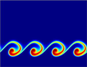
Figure 2 depicts the spatio-temporal distribution of the product  $C$ concentration obtained from our DNS in three different scenarios, namely when the chemical reaction produces a (a) less viscous (
 $R_{c}=-3$), (b) iso-viscous (
 $R_{c}=0$) and (c) more viscous (
 $R_{c}=3$) product. For
  $R_{c}=-3$, the IP in the base velocity profile (see figure 1e) is at the
  $B\unicode{x2013} C$ front, while
  $\bar {U}^{\prime \prime }$ moves away from zero to obtain a negative global minimum at the
  $C\unicode{x2013} A$ front. As a result, the flow-directed Kelvin–Helmholtz (KH) billows develop at the
  $B\unicode{x2013} C$ front, while the
  $C\unicode{x2013} A$ front has a stabilizing effect. Thus at a later dimensionless time (
 $t=30$), the
  $C\unicode{x2013} A$ front becomes almost flat, and the mixing occurs between
  $C$ and
  $B$ in the lower layer (see figure 2a). At this stage, the patterns in the lower layer resemble a cat-eye-type instability pattern reported in Roediger et al. (Reference Roediger, Kraft, Nulsen, Churazov, Forman, Brüggen and Kokotanekova2013). After a while, at
  $t=40$, under the reflexive lower boundary and vortex merging due to the complex nonlinear phenomenon, the
  $C\unicode{x2013} A$ front seems to have two crests and peaks. In the second scenario, i.e. for
  $R_{c}=0$, a stable RD front spreads transversely over time with no interfacial deformations (figure 2b). In the third scenario, i.e. for
  $R_{c}=3$, the base velocity profile exhibits an IP at the
  $C\unicode{x2013} A$ front. However,
  $\bar {U}^{\prime \prime }$ becomes negative at the
  $B\unicode{x2013} C$ front, albeit without having an IP (figure 1e). Thus the flow-directed roll-up-like patterns are formed at the
  $C\unicode{x2013} A$ front, while the
  $B\unicode{x2013} C$ front spreads stably without any deformation (figure 2c). For
  $R_{c}=3$, the region comprising fluids
  $C$ and
  $A$ can be regarded locally as a two-layer miscible non-reactive system, where a less-viscous fluid
  $A$ overlies a high-viscous fluid
  $C$, even though the product
  $C$ is generated due to the chemical reaction. Specifically, a comparison of our result shown inside the white dashed ellipse in figure 2(c) with the experimental result of Hu & Cubaud (Reference Hu and Cubaud2018) (see figure 2(a), zone (III), i.e. the inertial regime with a wavy interface of Hu & Cubaud Reference Hu and Cubaud2018) reveals that the
  $C\unicode{x2013} A$ front mimics almost the same patterns. It is noteworthy that if
  $Da=0$, then the present system of Eqs. (2.1) switches to the miscible non-reactive model of Hu & Cubaud (Reference Hu and Cubaud2018). Moreover, if the bottom fluid
  $B$ is more viscous than the upper fluid
  $A$, then the existence of zone (iv) of figure 2(a) of Hu & Cubaud (Reference Hu and Cubaud2018); i.e. the inertial regime with viscous ligament entrainment from wave crests, is confirmed as the Reynolds number increases. Also, if
  $R_{c}>0$, then similar ligament formations with over-topping of neighbour short waves are observed for the current reactive system (not shown here).

Figure 2. Spatio-temporal evolution of the product's concentration  $C$ for (a)
  $R_{c}=-3$, (b)
  $R_{c}=0$, (c)
  $R_{c}=3$, when
  $h=0.3$,
  $\delta =0.03$ (
 $t_{0}=0.34$),
  $Re=1000$,
  $Da=100$ and
  $Pe=2 \times 10^{4}$. (d) Interfacial lengths
  $I_{BC}$ (for
  $R_{c}=-3$) and
  $I_{CA}$ (for
  $R_{c}=3,0$) versus time.
Besides the destabilizing effect at the  $B\unicode{x2013} C$ front for
  $R_{c}<0$ (
 $C\unicode{x2013} A$ front for
  $R_{c}>0$) and the stabilizing effect at the
  $C\unicode{x2013} A$ front for
  $R_{c}<0$ (
 $B\unicode{x2013} C$ front for
  $R_{c}>0$), we notice that the interfacial deformation is severe for
  $R_{c}<0$ when compared to
  $R_{c}>0$. To analyse this quantitatively, we plot the interfacial length of the unstable fronts, i.e.
  $B\unicode{x2013} C$ for
  $R_{c}=-3$ (
 $I_{BC}$) and
  $C\unicode{x2013} A$ for
  $R_{c}=3$ (
 $I_{CA}$) in figure 2(d). Here,
  $I_{BC}=\iint _{\varOmega } |\boldsymbol {{\nabla } B}|\, {\textrm{d}\kern0.7pt x} \,{\textrm {d} y}$ and
  $I_{CA}=\iint _{\varOmega }|{\boldsymbol {\nabla } A}|\,\textrm{d}\kern0.7pt x\,\textrm {d}y$, where
  $\varOmega$ is the domain size. For
  $R_{c}=0$,
  $I_{BC}=I_{CA} \approx 4$ up to a final stopping time
  $t_{s} \ge 0$ before the horizontal diffusive interface reaches the top and bottom boundaries. Figure 2(d) also shows clearly that
  $I_{BC}$ for
  $R_{c}=-3$ attains a much greater value than that of
  $I_{CA}$ for
  $R_{c}=3$, and also starts to amplify early. This signifies that if the product's viscosity is less, then the instability onsets early and becomes more severe than in the case of a more-viscous product. These DNS results are limited to the initial disturbance (a sine wave at
  $y=h$) of a fixed wavenumber
  $\alpha =2{\rm \pi}$, so the growth quantified using
  $I_{BC}$ or
  $I_{CA}$ is based on a particular interfacial morphology. Moreover, the regularity of these multiple KH billows may be due to surpassing the most-unstable mode over all other modes of disturbances (Gallaire & Brun Reference Gallaire and Brun2017). Also, doubt is cast upon what is the band of wavenumbers for which the instability occurs.
The dispersion curves ( $\omega _i$ versus
  $\alpha$) obtained from LSA for different values of
  $R_{c}$ are shown in figure 3 for the same set of parameters as in figure 2. It can be seen that when
  $R_{c}=0$ (no viscosity stratification),
  $\omega _i<0$ for all
  $\alpha$, indicating that this situation is stable. Increasing
  $R_{c}$ to
  $R_{c}=0.5$, the disturbance becomes unstable (
 $\omega _i>0$) for
  $\alpha$ in the range
  $[5,10]$ (figure 3). Close inspection also reveals that the maximum growth rate
  $\omega _{i,max}$ occurs near
  $\alpha = 2{\rm \pi}$. In contrast, for
  $R_{c}=-0.5$, the band of unstable wavenumbers widens, with its
  $\omega _{i,max}$ larger than that for
  $R_{c}=0.5$. For
  $R_{c}=\pm 1$, the band of unstable wavenumbers increases, and the value of
  $\omega _{i,max}$ is higher for
  $R_{c}=-1$ than for
  $R_{c}=1$. Thus we can conclude that the growth rate of the disturbance is higher when
  $R_{c}<0$ as compared to
  $R_{c}>0$ with the same magnitude. In addition, figure 3 also shows the existence of stable wavenumbers in the presence of viscosity stratification.

Figure 3. Growth rate  $\omega _i = \textrm {Im}(\omega )$ versus
  $\alpha$ for various
  $R_{c}$, with
  $Da=100$,
  $h=0.3$,
  $\delta =0.03$ (
 $t_{0}=0.34$),
  $Re=1000$ and
  $Pe=2 \times 10^{4}$.
We summarize the obtained stable and unstable cases from LSA for any moderate  $Da$ and
  $R_{c}$ values, and compare them with the DNS results in figure 4. Figure 4(a) shows the variation of
  $R_{c}^{crit}$, which represents the minimum value of
  $R_{c}$ for which the growth rate becomes positive, with
  $Da$. A typical procedure to obtain
  $R_{c}^{crit}$ for a fixed
  $Da$ (
 $=40$) is shown as an inset in figure 4(a). It can be observed from this inset that increasing
  $R_{c}$ increases
  $\omega _{i,max}$ near the hump around
  $\alpha \approx 2{\rm \pi}$ in the dispersion curves, and it becomes positive for
  $R_{c}^{crit}=0.51$. Figure 4(a) reveals that as
  $Da$ increases,
  $R_{c}^{crit}$ decreases in magnitude for both positive and negative cases. However, this decrease in
  $R_{c}^{crit}$ is faster for
  $R_{c}<0$ than for
  $R_{c}>0$. Thus the
  $Da\unicode{x2013} R_{c}^{crit}$ plane in figure 4(a) shows a stable region around
  $R_{c}=0$, which is sandwiched between two unstable regions in an asymmetric fashion. Also, for a fixed
  $Da$, if
  $R_{c}>0$, then
  $R_{c}^{crit}$ has a higher magnitude compared to that of
  $R_{c}<0$. So the unstable region to the left of
  $R_{c}=0$ covers more area than the unstable region to the right of
  $R_{c}=0$.

Figure 4. (a) The  $Da\unicode{x2013} R_{c}^{crit}$ plane obtained from the LSA; inset shows typical dispersion curves for
  $Da=40$,
  $R_{c}>0$, where
  $R_{c}^{crit}=0.51$. Density plots of
  $C$ for various
  $Da$, with (b)
  $R_{c}=-3$ (at
  $t=12$), (c)
  $R_{c}=3$ (at
  $t=40$). (d) The
  $Da\unicode{x2013} R_{c}^{crit}$ plane obtained from the DNS; insets show the zoomed density plot of
  $C$ in stable and unstable regions. The common parameters are
  $h=0.3$,
  $\delta =0.03$,
  $Re=1000$ and
  $Pe=2 \times 10^{4}$.
The LSA may not always predict the most unstable mode of the perturbation, but it is an effective method that enables us to rationalize some of the flow features qualitatively (Gallaire & Brun Reference Gallaire and Brun2017). Here, as we see from LSA, for the critical  $R_{c}^{crit}$, the maximal growth occurs around the wavenumber
  $\approx 2{\rm \pi}$, and we use a sine wave of this wavenumber to perturb the initial condition in the DNS and solve the nonlinear problem. In figure 4(b), we show the colour density profiles of the product's concentration for
  $R_{c}=-3$ at
  $t=12$ with increasing
  $Da$. As predicted by the LSA, the interfacial deformation by the KH billows is more notable for a larger value of
  $Da$. Similar monotonic behaviour is also noticed for
  $R_{c}=3$ (see figure 4c). To compare these observed effects with LSA results (figure 3), we differentiate the stable and unstable region in the
  $Da\unicode{x2013} R_{c}^{crit}$ plane again by measuring the interfacial lengths. In DNS, we run a search algorithm that assigns a set of parameters
  $(Da, R_c )$ as unstable ones if the corresponding interfacial length (
 $I_{BC}$ for
  $R_{c}<0$, and
  $I_{CA}$ for
  $R_{c}>0$) exceeds the reference value
  $4$. Otherwise, we assign them as a stable pair. In this way, we obtain the
  $R_{c}^{crit}$ values for various
  $Da$ and plot them in figure 4(d). Strikingly similar asymmetric behaviour is noticed as in LSA. The typical stable and unstable patterns are shown as insets in figure 4(d) to differentiate the dynamics.
In Figure 5(a), we plot the boundary curves obtained from LSA that separate the stable and unstable zones in the  $Da\unicode{x2013} R_{c}^{crit}$ plane for varying
  $Pe$. As
  $Pe$ decreases, the unstable zones shrink for both
  $R_{c}<0$ and
  $R_{c}>0$, indicating that the flow is less unstable for a lower
  $Pe$. Since
  $Pe= Re \,Sc$ (where
  $Sc={\mu _{1}}/{\rho D}$ is the Schmidt number, and
  $Re={\rho Q}/{\mu _{1}}$), a change in
  $Pe$ means that the variation is only in
  $Sc$ as the Reynolds number is fixed. So the decrease in
  $Pe$ means that the diffusion dominates more over the momentum transfer due to viscosity, resulting in a more stable flow. Also, the gaps between the different boundaries for different
  $Pe$ are less for
  $R_{c}<0$ than for
  $R_{c}>0$. This shows that a change in
  $Pe$ influences the stability of the flow more for
  $R_{c}>0$ as compared to
  $R_{c}<0$. Again, we define
  $R_{c}^{-}=R_{c}^{crit}/(80\,Pe^{-0.4})$ when
  $R_{c}<0$, and
  $R_{c}^{+}=R_{c}^{crit}/(350\,Pe^{-0.54})$ when
  $R_{c}>0$, by a naive observation of the correlation between the critical values for different
  $Pe$. Then we plot these boundaries in the
  $Da\unicode{x2013} R_{c}^{-}$ plane and the
  $Da\unicode{x2013} R_{c}^{+}$ plane in figures 5(b) and 5(c), respectively. It is clear that these scales merge the boundary between stable and unstable zones for different
  $Pe$. This implies that the stability can be made independent of the changes in solute diffusion by using these scales. Moreover, the redefined boundaries follow the relations
  $-0.24 (R_{c}^{-})^{\eta ^{-}}-0.12$ (see the blue solid line in figure 5b) and
  $(R_{c}^{+})^{\eta ^{+}}+0.01$ (see the red solid line in figure 5c), where
  $\eta ^{-}=-0.58$ and
  $\eta ^{+}=-0.31$. Clearly,
  $\eta ^{-}<\eta ^{+}$ means that if
  $Da$ increases, then
  $R_{c}^{crit}$ decreases for
  $R_{c}<0$ at a faster rate than for
  $R_{c}>0$. Thus it signifies an asymmetric sandwiching of the stable zone between the unstable zones with a larger instability region for cases with
  $R_{c}<0$ rather than
  $R_{c}>0$. In figures 5(d,e), we validate the predicted results of LSA with DNS by showing the density of the product's concentration when
  $R_{c}=-3$ (at
  $t=40$) and
  $R_{c}=3$ (at
  $t=50$), respectively, for various
  $Pe$. For both
  $R_{c}=-3$ and
  $R_{c}=3$, the interfacial deformations increase with increasing
  $Pe$, which agrees with the LSA predictions.

Figure 5. (a) The  $Da\unicode{x2013} R_{c}^{crit}$ plane for various
  $Pe$ obtained from the LSA. (b) The
  $Da\unicode{x2013} R_{c}^{-}$ plane, where
  $R_{c}^{-}=R_{c}^{crit}/(80\,Pe^{-0.4})$ and the boundary curve that follows
  $-0.24(R_{c}^{-})^{\eta ^{-}}-0.12$, where
  $\eta ^{-}=-0.58$. (c) The
  $Da\unicode{x2013} R_{c}^{+}$ plane, where
  $R_{c}^{+}=R_{c}^{crit}/(350\, Pe^{-0.54})$ and the boundary curve that follows
  $(R_{c}^{+})^{\eta ^{+}}+0.01$, where
  $\eta ^{+}=-0.31$. The density plots of
  $C$ for various
  $Pe$ with (d)
  $R_{c}=-3$ (at
  $t=40$), (e)
  $R_{c}=3$ (at
  $t=50$), when
  $h=0.3$,
  $\delta =0.03$,
  $Re=1000$ and
  $Da=100$.
4. Conclusions
Despite its tremendous importance to industrial economics in terms of recovery costs if suppressed or even reduced by only a few percent, the chemo-hydrodynamic instabilities in the vicinity of viscosity stratification remained underdog and not studied in the Navier–Stokes regime (Govindarajan & Sahu Reference Govindarajan and Sahu2014; De Wit Reference De Wit2020). We found that a  $A+B \rightarrow C$ type reaction generates KHI patterns at both reactive fronts by creating favourable IPs through a local viscosity modification in a layered channel flow. One such pattern is analogous to that observed in the experiment of Hu & Cubaud (Reference Hu and Cubaud2018). Both our LSA and DNS results demonstrate that the
  $Da\unicode{x2013} R_{c}^{crit}$ plane has an asymmetric property, indicating that the flow is more unstable if the reaction's product is less viscous. The flow is more unstable for a higher Péclet number, and the stability can eliminate the changes in solute diffusion by using appropriate scales.
Funding
M.M. acknowledges the financial support from SERB, Government of India through project grant no. CRG/2020/000613. M.M. also gratefully acknowledges the financial support of the project grant of SPARC (P-450), Government of India. K.C.S. thanks SERB, Government of India, for their financial support through grant no. CRG/2020/000507. S.N.M. also acknowledges the support of UGC, Government of India, with a research fellowship.
Declaration of interests
The authors report no conflict of interest.


