2.1. Governing equations of flow

The 3-D incompressible, unsteady flow around the prism is modelled by the filtered Navier–Stokes equations:

(2.1)\begin{gather}\frac{{\partial {{\bar{u}}_i}}}{{\partial {x_i}}} = 0,\end{gather}

(2.2)\begin{gather}\frac{{\partial {{\bar{u}}_i}}}{{\partial t}} + \frac{{\partial {{\bar{u}}_i}{{\bar{u}}_j}}}{{\partial {x_j}}} ={-} \frac{1}{\rho }\frac{{\partial \bar{p}}}{{\partial {x_i}}} + \frac{\partial }{{\partial {x_j}}}\left( {\nu \frac{{\partial {{\bar{u}}_i}}}{{\partial {x_j}}} - {\tau_{ij}}} \right),\end{gather}

where the overbar stands for the spatial filter operation; x_i denotes the ith Cartesian coordinate, u_i denotes the velocity component in the direction x_i, t is time, p is pressure, ρ is fluid density, ν is kinematic viscosity and ${\tau _{ij}} = \overline {{u_i}{u_j}} - {\bar{u}_i}{\bar{u}_j}$ is the subgrid-scale stress and is modelled by the dynamic k-equation model developed by Yoshizawa (Reference Yoshizawa1986).

The governing equations are solved by the open-source finite-volume code OpenFOAM. The implicit second-order backward differentiation scheme is adopted for temporal integration. The so-called Gauss limited linear scheme, a second-order-accurate bounded total variational diminishing scheme, is used for spatial discretization of the convection term, while the second-order central difference scheme is used for the diffusion term. The gradient term is evaluated using the least-squares method. The velocity–pressure coupling is achieved by the pressure-implicit with splitting of operators (PISO) algorithm with two correctors in each time step. The convergence criterion for p is 1 × 10⁻⁶.

2.2. Simulation cases

Figure 1 shows a schematic diagram of the numerical cases simulated in this study. First, rectangular prisms with B/D values ranging from 3 to 12, with a unit interval, are used to investigate the variations of the flow characteristics with B/D. In particular, the critical value of B/D at which the flow pattern jumps from the first mode (St = 0.6) to the second mode (St = 1.2) is explored. Furthermore, two special configurations are presented to separate the ILEV and TEVS. Case II is characterized by a splitter plate in the wake to eliminate the TEVS. In Case III, the leading-edge separated shear layer is removed, and only TEVS is expected to occur. This is equivalent to a prism of infinite width, where the interactions between the ILEV and TEVS are negligible and the TEVS can be analysed separately.

Figure 1. Simulation cases. Case I represents regular rectangular prisms. Case II and Case III are designed to separate the ILEV and TEVS.

2.3. Computational domain, boundary conditions and mesh arrangement

Figure 2 shows a schematic view of the computational domain and boundary conditions for the regular prisms (i.e. Case I in figure 1). The distances from the prism centre to the inlet and outlet boundary are 50D and 150D, respectively. The transverse dimension of the computational domain is 100D, resulting in a blockage ratio of 1%. The spanwise dimension, i.e. the prism length L, is set as 5D, which is determined based on a comparison with 10D in § 2.4.

Figure 2. Computational domain and boundary conditions for Case I.

A uniform flow velocity U is specified at the inlet boundary. At the outlet boundary, the Dirichlet boundary condition (zero value) is used for pressure, while the Neumann boundary condition (zero gradient) is used for velocity. The top and bottom boundaries are set as symmetry, while the front and back boundaries are periodic. No-slip wall boundary is applied to the prism surface. Similar strategies are adopted for Cases II and III and not given herein for brevity.

The mesh in the x–y plane is hybrid, with 20 layers of structured grids around the prism and unstructured quadrilateral grids in the rest of the domain, as shown in figure 3 for B/D = 5. To solve the small-scale vortex structures around the prism, the grids in the near-wall and near-wake regions are refined. The grid size within the structured region is 0.02D × 0.02D, leading to a unit grid aspect ratio and an average y ⁺ about 1.0 and a maximum y ⁺ about 3.0 during simulations. The grid spacing gradually increases away from the wall. In figure 3(b), the grid size at the perimeter of the white rectangle (7D downstream of the prism's rear face and 2D from other faces) is 0.05D.

Figure 3. Mesh arrangement around the prism with B/D = 5: (a) 20 layers of structured mesh in body vicinity; (b) unstructured mesh in the rest area.

The 3-D mesh is obtained by extruding the two-dimensional (2-D) mesh in the x–y plane along the spanwise direction with a uniform step size (δz). In the present study, δ = 0.05D is adopted following a dependence study on δz (see § 2.4). This leads to 100 layers in the spanwise direction for the 3-D mesh. The total cell number for regular prisms varies from 9.6 million (B/D = 3) to 15.1 million (B/D = 12). For Cases II and III, there are 15.7 million and 10.5 million cells, respectively.

2.4. Mesh resolution and spanwise domain size

It is known that mesh resolution, in both the x–y plane and the spanwise direction, and the spanwise domain size may have significant influences on the simulated flow around a rectangular prism (Bruno, Coste & Fransos Reference Bruno, Coste and Fransos2012; Zhang & Xu Reference Zhang and Xu2020). In the present study, a mesh dependence study is performed. Based on the reference mesh introduced in § 2.3, which is labelled as Case (i), three variations are examined:

1. (ii) The L value is increased from 5D to 10D.

2. (iii) The δz value is decreased from 0.05D to 0.025D.

3. (iv) The δx and δy values in the inner zone are decreased from 0.02D to 0.01D.

Detailed mesh arrangements for the four cases are listed in table 1. For Cases (i)–(iii), the non-dimensional time step size δt* = δt ⋅ U/D is set as 0.01, where δt is the physical time step size. While for Case (iv), δt* is 0.005. The maximum Courant number is below 1.2. Each simulation lasts 600 non-dimensional time units, while the data in the first 300 time units are discarded to exclude the initial undeveloped flow period.

Table 1. Simulated aerodynamic force coefficients and St with different mesh arrangements.

Table 1 lists the Strouhal number, the time-averaged drag coefficient (C_D-avg) and the standard deviation of lift coefficient (C_L-std) obtained from different arrangements. The Strouhal number is defined as

(2.3)\begin{equation}St = \frac{{fB}}{U},\end{equation}

where f is the peak frequency of the unsteady lift coefficient and is calculated by the fast Fourier transform (FFT) technique. The drag and lift coefficients are defined as

(2.4a)\begin{gather}{C_D} = \frac{{{F_D}}}{{0.5\rho {U^2}DL}},\end{gather}

(2.4b)\begin{gather}{C_L} = \frac{{{F_L}}}{{0.5\rho {U^2}DL}},\end{gather}

where F_D and F_L are the unsteady drag and lift forces, respectively. It can be found that the aerodynamic force coefficients calculated from different cases are fairly close. The error of C_L-std is relatively large, while the key parameter of this study, i.e. St, stays almost constant.

The time-averaged value (C_p-avg) and standard deviation (C_p-std) of the surface pressure coefficients are plotted in figure 4. Data are averaged along the spanwise direction and between the top and bottom surfaces. In general, the influences of L and δz are very limited. For C_p-avg, the four curves almost coincide with each other. For C_p-std, the deviations of the peak value from Case (i) are within 5%.

Figure 4. Spanwise- and side-averaged pressure coefficients on the lateral faces with different mesh arrangements.

To check the mesh convergence of velocity fields around the prism, the time-varying velocities at two columns of probes at x/D = 0 and 3.5 are monitored, as shown in figure 5(a). The spanwise location of the probes is z = 0 (midspan). Figures 5(b) and 5(c) display the time-averaged (U-avg) and standard deviations (U-std) of the velocity profile along x/D = 0 and 3.5, respectively. For both regions, different mesh arrangements give close estimates of U-avg and U-std. Thus, it can be concluded that the meshing parameters for Case(i), i.e. L = 5D and δz = 0.05D, can give a nearly converged estimation of the main flow features and are therefore adopted for the following simulations.

Figure 5. Midspan velocity profiles with different mesh arrangements: (a) probe locations; (b) x/D = 0; (c) x/D = 3.5.

3.1. The DMD algorithm

For a linear system, ${\boldsymbol{x}^{n + 1}} = \boldsymbol{\mathsf{A}}{\boldsymbol{x}^n}$, if the eigenvalues and eigenvectors of the coefficient matrix $\boldsymbol{\mathsf{A}}$ are determined, one can obtain the main evolution characteristics of the system. In the present study, the DMD method proposed by Schmid (Reference Schmid2010) is used for the eigenvalue decomposition of matrix $\boldsymbol{\mathsf{A}}$.

First, by consecutively sampling the system at an interval of δt, the data can be arranged into a snapshot matrix:

(3.1)\begin{equation} \boldsymbol{\mathsf{X}} = (\boldsymbol{x}({t_1}),\boldsymbol{x}({t_2}), \ldots ,\boldsymbol{x}({t_n})),\end{equation}

where each column denotes an instantaneous snapshot of the system. For an unsteady pressure field, $\boldsymbol{\mathsf{X}}$ is expressed as follows:

(3.2) \begin{equation} \boldsymbol{\mathsf{X}} = \left( \begin{array}{@{}cccc@{}} {{p_{nod{e_1}}}({t_1})}&{{p_{nod{e_1}}}({t_2})}& \cdots &{{p_{nod{e_1}}}({t_n})}\\ {{p_{nod{e_2}}}({t_1})}&{{p_{nod{e_2}}}({t_2})}& \cdots &{{p_{nod{e_2}}}({t_n})}\\ \vdots & \vdots & \ddots & \vdots \\ {{p_{nod{e_k}}}({t_1})}&{{p_{nod{e_k}}}({t_2})}& \cdots &{{p_{nod{e_k}}}({t_n})} \end{array} \right),\end{equation}

where node ₁–node_k denote the spatial dimension of the flow fields, i.e. the number of degrees of freedom, while t ₁–t_n denote the temporal dimension, i.e. the sampling length. Similarly, one can construct another matrix:

(3.3)\begin{equation}\boldsymbol{\mathsf{Y}} = (\boldsymbol{x}({t_2}),\boldsymbol{x}({t_3}), \ldots ,\boldsymbol{x}({t_{n + 1}})),\end{equation}

where $\boldsymbol{\mathsf{Y}}$ = $\boldsymbol{\mathsf{AX}}$.

Second, the singular value decomposition or the proper orthogonal decomposition (POD) of $\boldsymbol{\mathsf{X}}$ is computed as follows:

(3.4)\begin{equation} \boldsymbol{\mathsf{X}} = \boldsymbol{\mathsf{USV}}^\ast,\end{equation}

where $\boldsymbol{\mathsf{U}}$ contains the POD modes of the system and $\boldsymbol{\mathsf{S}}$ represents the energetic importance of each mode. To reduce the computational cost, only the first r order modes are retained to approximate the original flow fields: $\boldsymbol{\mathsf{Ur}} = \boldsymbol{\mathsf{U}}(1:k,1:r)$, $\boldsymbol{\mathsf{Sr}} = \boldsymbol{\mathsf{S}}(1:r,\; 1:r)$ and $\boldsymbol{\mathsf{Vr}} = \boldsymbol{\mathsf{V}}(1:n,1:r)$. In this study, it is found that the first 100 order POD modes contain more than 95% of the energy of the original flow fields, and the DMD spectra calculated based on the first 100 and 200 POD modes are very close. Thus, r = 100 is adopted for computational efficiency.

Third, $\boldsymbol{\mathsf{X}} = \boldsymbol{\mathsf{Ur}}\boldsymbol{\mathsf{Sr}}\boldsymbol{\mathsf{Vr}}^\ast$ is substituted into $\boldsymbol{\mathsf{Y}}$ = $\boldsymbol{\mathsf{AX}}$, and then $\boldsymbol{\mathsf{A}}$ can be expressed as follows:

(3.5)\begin{equation} \boldsymbol{\mathsf{A}} = \boldsymbol{\mathsf{Y}}\boldsymbol{\mathsf{Vr}} \boldsymbol{\mathsf{Sr}}^{-1}\boldsymbol{\mathsf{Ur}}^\ast.\end{equation}

Although matrix $\boldsymbol{\mathsf{A}}$ is obtained, it has an order of k × k, which means that a direct eigenvalue decomposition of $\boldsymbol{\mathsf{A}}$ is extremely difficult for large-scale systems. An alternative approach is to reduce the order by projecting $\boldsymbol{\mathsf{A}}$ onto $\boldsymbol{\mathsf{Ur}}$:

(3.6) \begin{equation} \tilde{\boldsymbol{\mathsf{A}}} = \boldsymbol{\mathsf{Ur}}^\ast \boldsymbol{\mathsf{A}}{\boldsymbol{\mathsf{Ur}}} = \boldsymbol{\mathsf{Ur}}^\ast ({\boldsymbol{\mathsf{Y}}}{\boldsymbol{\mathsf{Vr}}}\boldsymbol{\mathsf{Sr}}^{ - 1} \boldsymbol{\mathsf{Ur}}^\ast ){\boldsymbol{\mathsf{Ur}}} = \boldsymbol{\mathsf{Ur}}^\ast {\boldsymbol{\mathsf{Y}}}{\boldsymbol{\mathsf{Vr}}}\boldsymbol{\mathsf{Sr}}^{ - 1}.\end{equation}

Note that the order of $\tilde{\boldsymbol{\mathsf{A}}}$ is only r × r, and performing eigenvalue decomposition for $\tilde{\boldsymbol{\mathsf{A}}}$ is very efficient:

(3.7)\begin{equation}[\boldsymbol{\mathsf{W}},\boldsymbol{\varLambda}] = \textrm{eig}(\tilde{\boldsymbol{\mathsf{A}}}).\end{equation}

Here $\boldsymbol{\mathsf{A}}$ and $\tilde{\boldsymbol{\mathsf{A}}}$ are similar matrices, and thus they share the same eigenvalues: λ_i = diag($\boldsymbol{\varLambda}$). The eigenvalues of the DMD modes can then be calculated by ω_i = log(λ_i)/δt. The real part of ω_i denotes the growth rate of the ith mode, while the imaginary part denotes the oscillating frequency. For the eigenvectors, i.e. the DMD modes, Tu et al. (Reference Tu, Rowley, Luchtenburg, Brunton and Kutz2013) pointed out that there are two kinds of definitions. The first is the projected DMD mode:

(3.8)\begin{equation}\hat{\boldsymbol{\varPhi}} = \boldsymbol{\mathsf{UW}}.\end{equation}

The second is the exact DMD mode:

(3.9)\begin{equation}\boldsymbol{\varPhi} = \boldsymbol{\mathsf{Y}}\boldsymbol{\mathsf{V}}{\boldsymbol{\varLambda}^{ - 1}}\boldsymbol{\mathsf{W}}.\end{equation}

In this study, the exact DMD mode is adopted for the following analyses. Like the eigenvalues, the DMD modes are also in complex form. For a specific mode ${\boldsymbol{\varphi }_i} = {({x_1} + \textrm{i}{y_1},{x_2} + \textrm{i}{y_2}, \ldots ,{x_k} + \textrm{i}{y_k})^\textrm{T}}$, the phase angle at each spatial point can be calculated by

(3.10)\begin{equation}\theta _i^k = \textrm{arctan}\left( {\frac{{{y_k}}}{{{x_k}}}} \right).\end{equation}

Based on the distribution of the phase angle in the entire domain, a more direct understanding of the fluctuating behaviour of the instability mode can be obtained.

Finally, based on the eigenvalues and eigenvectors, the flow evolution corresponding to a specific DMD mode can be reconstructed:

(3.11)\begin{equation}{\boldsymbol{x}_i}(t) = \boldsymbol{\varphi }_i^\textrm{T}\boldsymbol{x}({t_1})\,{\textrm{e}^{{\omega _i}(t - {t_1})}}{\boldsymbol{\varphi }_i} = {\psi _i}(t){\boldsymbol{\varphi }_i},\end{equation}

where ${\psi _i}(t) = \boldsymbol{\varphi }_i^\textrm{T}\boldsymbol{x}({t_1})\,{\textrm{e}^{{\omega _i}(t - {t_1})}}$ represents the temporal coefficient of mode ${\boldsymbol{\varphi }_i}$.

Although the derivation above is based on a linear system, Rowley et al. (Reference Rowley, Mezić, Bagheri, Schlatter and Henningson2009), Tu et al. (Reference Tu, Rowley, Luchtenburg, Brunton and Kutz2013) and Mezić (Reference Mezić2013) pointed out that the DMD algorithm is also applicable to nonlinear systems by revealing its relationship with the Koopman operator. To obtain satisfactory results, Schmid (Reference Schmid2010) noted that the sampling frequency should be at least three times the inherent frequency. The DMD algorithm for vector fields, such as the velocity field, is similar to that for a scalar field, with the only exception that each component of the vector should be treated as an individual degree of freedom and then arranged into an integral snapshot matrix.

Unlike the POD approach where the modes are arranged in the order of energy contents, there is no objective ranking of the eigenvalues in the DMD approach; thus it is difficult to determine the most physically relevant modes. In this study, the main modes which are related to the flow global instability are identified through the following guidelines. First, the global instability is expected to be caused by the self-sustained oscillations of the shear layer and periodic shedding of the TEVS, and thus the growth rate of concerned modes should be close to zero, provided that the sampling length is large enough. Second, the spectrum of the lift force provides a direct reference for the selection of the DMD mode by comparing the frequencies. Third, the DMD modes directly obtained by (3.9) are first normalized based on the magnitude, and the time-varying coefficient ψ(t) of each mode can be calculated, then the modes are reordered by their 2-norm of ψ(t). The mode with higher ${\parallel} \psi (t)\parallel$ represents higher energy and is more likely to be the dominant mode of the global instability.

3.2. Two-dimensionality of DMD mode of global instability

The sampling length and frequency play significant roles in the decomposition accuracy. Thus, a large number of snapshots are usually needed to be stored when constructing matrix $\boldsymbol{\mathsf{X}}$. If the target is the 3-D flow fields, it will require a large amount of memory and computational time to perform the DMD analysis, which may be prohibitive in most cases. The emphasis of this study is to examine the streamwise evolution of the vortices dominating the global instability. If the 3-D fluctuations can be expressed by a 2-D slice in the x–y plane, the computational effort will be significantly reduced. Thus, in this section, the effectiveness of the 2-D DMD for extracting the global instability structures is examined through the DMD mode of the pressure coefficients on the top surface of the prism.

Two prisms, i.e. B/D = 5 and 6, are examined, which correspond to scenarios where one and two vortices exist on each lateral side of the prism, respectively, according to Nakamura et al. (Reference Nakamura, Ohya and Tsuruta1991). There are in total 40 000 snapshots for each case, and the time interval between two consecutive snapshots is 0.01, corresponding to about 46 and 70 vortex shedding periods, respectively. The spectra of the DMD eigenvalues are depicted in figure 6, where the abscissa and ordinate represent the imaginary and real parts of ω_i, respectively. The areas of the circles are scaled by ||ψ(t)||.

Figure 6. Dynamic mode decomposition spectra of the surface pressure for: (a) B/D = 5 and (b) B/D = 6. The areas of the circles are related to the energy of the modes.

From the spectra, the relatively stable (real (ω_i) ≈ 0) and high-energetic modes can be easily identified. The real and imaginary parts of the first mode marked in the figure are close to zero, representing zero growth and no oscillations. Thus, the first mode represents the time-averaged pressure field. Apart from the first mode, the second modes have the second largest area and are closest to the real (ω_i) = 0 axis. The values of St calculated by the eigenvalues of the second modes for the two prisms are 0.571 and 1.062, respectively. The results calculated using the FFT of C_L are 0.576 and 1.064, respectively, suggesting that the second modes are essentially the global instability modes. For the sake of brevity, the global instability mode is referred to as the St mode hereafter. The spectra are symmetric about the imaginary (ω_i) = 0, i.e. a pair of conjugate modes exists for each non-zero frequency. Figure 7 shows the pressure distributions of the first mode and the real and imaginary parts of the second mode for the two prisms. It should be noted that figure 7 only shows the shape of a specific DMD mode, i.e. ${\boldsymbol{\varphi }_i}$ in (3.11). The absolute value of the pressure fluctuations corresponding to a specific mode ${\boldsymbol{\varphi }_i}$ can be obtained by multiplying its time-varying coefficient ${\psi _i}(t)$. The imaginary part has a ${\rm \pi}$/2 phase lag relative to the real part. Thus, it can be inferred that the global instability mode has a travelling-wave form, consistent with the physical background of the vortex shedding behaviour associated with the global instability.

Figure 7. Dynamic mode decomposition modes of surface pressure: (a) B/D = 5, first mode; (b) B/D = 5, second mode, real part; (c) B/D = 5, second mode, imaginary part; (d) B/D = 6, first mode; (e) B/D = 6, second mode, real part; ( f) B/D = 6, second mode, imaginary part.

As shown in figure 7, the first and second modes both show strong correlations in the spanwise direction, suggesting that the surface pressure fluctuations are mainly governed by the streamwise evolution of the vortices.

In addition, DMD is performed on the 3-D velocity fields to further check the 2-D features of the global vortex shedding modes. The vortical structures within the velocity DMD modes are identified based on the iso-surfaces of the Q criteria, as shown in figure 8 for B/D = 5 and 6. Here Q is defined as

(3.12)\begin{equation}Q = {\textstyle{1 \over 2}}(\|{\boldsymbol{\varOmega}\| ^2} - {\|\boldsymbol{\mathsf{S}}\|^2}),\end{equation}

where S and Ω are the symmetric and antisymmetric components of the velocity gradient tensor, respectively. Parameter Q represents the local balance between shear strain rate and vorticity magnitude. Positive Q corresponds to the rotational motion of the flow, and higher Q means higher vortex intensity. These Q criteria are considered to be more appropriate than the vorticity criteria for extracting vortex structures, especially in the near-wall region where the shear effect in the flow is predominant.

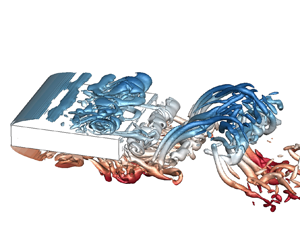
Figure 8. Global instability modes identified from the 3-D velocity fields: (a) B/D = 5; (b) B/D = 6. Vortical structures are demonstrated by iso-surfaces of Q = 0.2(U/D)², blue tubes have a clockwise direction of rotation and red tubes have an anti-clockwise direction of rotation.

From figure 8, several spanwise vortex tubes are observed on the lateral sides of and in the wake of the prisms, indicating that the global vortex shedding is almost synchronous along the spanwise direction. This permits us to use the 2-D flow fields in the x–y plane for the following DMD analyses to avoid high computational efforts. In the present study, the spanwise-averaged flow is used for the 2-D DMD analysis because it contains more averaged information than a slice in the 3-D flow. Detailed discussion on the evolution of the vortical structures of the DMD modes is given in § 4.2.

4.1. Formation of leading- and trailing-edge vortices

The instantaneous coherent structures of the 3-D flow fields during one vortex shedding cycle are extracted based on the Q iso-surfaces, as shown in figure 9.

Figure 9. (a–i) Evolution of coherent structures during one vortex shedding cycle for B/D = 5, demonstrated by iso-surfaces of Q = 1.0(U/D)², coloured based on the y coordinate.

At t = 0, a large-scale leading-edge vortex and a Kármán-like trailing-edge vortex appear above the top face and behind the leeward face, respectively. For brevity, in the text below, the leading- and trailing-edge vortices are referred to as the L and T vortices, respectively. At t = T/8, accompanied by the shedding of the L and T vortices, a small-scale spanwise vortex structure emerges in the leading-edge shear layer, which is caused by the Kelvin–Helmholtz (KH) instability. During the whole period, there are three KH rollers on the upper side, which are shed from the leading-edge shear layer at t/T = 1/8, 4/8 and 6/8. The downstream convection velocity of the first KH roller gradually decreases after being shed, promoting its subsequent coalescence with the second and third KH rollers at t = 5T/8 and T, respectively. The merger of the KH rollers in the leading-edge separation bubble was also detected by Sasaki & Kiya (Reference Sasaki and Kiya1991), Hwang, Sung & Hyun (Reference Hwang, Sung and Hyun2000) and Chaurasia & Thompson (Reference Chaurasia and Thompson2011) for a blunt flat plate at relatively low Reynolds numbers (Re < 800). In particular, Sasaki & Kiya (Reference Sasaki and Kiya1991) noted that the number of the merging KH rollers increased with Re. The merged large-scale vortex structure at t = T is actually the new L vortex and then propagates through the trailing edge over t/T ~ 1/4 to 3/4 in the next cycle. For the remaining half-cycle from 3T/4 to T + T/4, a relatively small T vortex is formed near the upper trailing edge without the influence of the large L vortex. During shedding, convection and coalescence, the KH rollers experience notable spanwise modulations. Furthermore, the L vortex is stretched to 3-D hairpin-like vortices when it flows past the trailing edge due to the strong shear effect near the wall.

Figure 10 shows the instantaneous coherent structures during one shedding cycle for B/D = 6. In contrast to the case of B/D = 5 shown in figure 9, every two KH rollers merge together and form the ILEV for B/D = 6, suggesting that the number of shedding KH rollers in one cycle is related to B/D. In addition, two large-scale vortices appear over the chord in figure 10, indicating a transition of the global instability from Mode 1 to Mode 2. However, the Kármán-type vortex shedding from the trailing edge is almost invisible. The underlying mechanism for such a mode transition is discussed in detail in § 5.2.

Figure 10. (a–i) Evolution of coherent structures during one vortex shedding cycle for B/D = 6, demonstrated by iso-surfaces of Q = 1.0(U/D)², coloured based on the y coordinate.

To better study the relationship between the KH instability and global instability, we defined a probe A in the upper shear layer and sampled the fluctuating velocity at that point. The probe is located at the midspan (z = 0) and is 2D downstream from the leading edge, as shown in figure 11. The heights of the probe for B/D = 5 and B/D = 6 are 0.55D and 0.58D, respectively, which correspond to the upper boundary of the mean separation bubble.

Figure 11. Locations of sampling probe A in the shear layer for (a) B/D = 5 and (b) B/D = 6.

Figure 12 shows the spectra of the normalized transverse velocity U_y/U ₀ at point A for B/D = 5 and 6. To facilitate comparison, the frequency is scaled by D rather than B. Several prominent peaks appear in both cases, including the global instability frequency, f_G, its harmonics, 2f_G and 3f_G, and the KH instability frequency, f_KH. Side-band frequencies of f_KH + f_G and f_KH + 2f_G also appear in the case of B/D = 5, which is expected to be caused by the nonlinear interactions between the large-scale vortex structures and the KH rollers. The f_KH in the case of B/D = 5 is close to 3f_G, in accordance with the coalescence of every three KH rollers during one shedding cycle of the large-scale vortex observed in figure 9. In contrast, f_KH is closer to 2f_G for B/D = 6. Thus, two KH rollers merge together during one shedding cycle in figure 10. It is worth noting that the f_KH values in the two cases are similar (around 0.4), and the decrease for f_KH/f_G for B/D = 6 is caused by the increase in f_G as a result of the mode transition of the global instability. In figure 12(b), the transverse velocity at the frequency of f_KH is lower than that in figure 12(a). The reason may be that the f_G value for B/D = 6 is much higher than that for B/D = 5, and the KH rollers are less developed before their merger into a large-scale leading-edge vortex. Thus, the KH instability for B/D = 6 is weaker than that for B/D = 5.

Figure 12. Spectra of the transverse velocity at point A in the shear layer for (a) B/D = 5 and (b) B/D = 6.

Figures 9 and 10 show that the subsequent shedding and merging of a certain number of KH rollers in the leading-edge shear layer are the source of the ILEV. How the KH instability, which has a significantly lower fluctuation amplitude in the spectra, forms the large-scale instability of ILEV remains unclear. To determine this, the time histories of U_y/U ₀ at probe A at two spanwise locations and their time-frequency spectra computed using the Morlet wavelet transform (Kijewski & Kareem Reference Kijewski and Kareem2003) are presented in figure 13. Several ‘packets' of high-frequency fluctuations, which correspond to the KH instability, can be observed. The inset in figure 13(a) shows a close-up view of the first ‘packet’ over t = 500–550. The amplitudes of the high-frequency fluctuations in these ‘packets' are much larger than those for the primary shedding frequency, indicating that the KH rollers contain a large amount of energy to be transferred to the ILEV. Nevertheless, the high-frequency fluctuations appear only intermittently, making them less apparent in the long-time-averaged velocity spectra and leading to a broad-band peak at f_KH in figure 12. It is worth noting that these large-amplitude ‘packets’ of high-frequency fluctuations exist for all B/D values. Cimarelli, Leonforte & Angeli (Reference Cimarelli, Leonforte and Angeli2018) studied the relationship between the low-frequency unsteadiness of the separation bubble and the small-scale structures in the shear layer based on direct numerical simulations for a 5:1 rectangular cylinder. They noted that the low-frequency unsteadiness alternatively promotes and suppresses the small-scale motions with a relatively long period of inversion, which further leads to the rising of the ‘packets’ of high-frequency fluctuations.

Figure 13. Time histories and time–frequency spectra of the transverse velocity of point A at z = 0 (a,b) and z = −1.5D (c,d) for B/D = 5.

From figures 13(a) and 13(c), it can be noticed that the amplitudes and locations of the ‘packets’ of high-frequency fluctuations show significant differences between z = 0 and −1.5D, suggesting that the KH instabilities at different locations are not enhanced or suppressed simultaneously. In addition, it can be directly observed from figures 9 and 10 that the KH rollers are not fully correlated in the spanwise direction. Thus, it is surmised that the intermittency of KH instability is mainly caused by the 3-D disturbance in the flow on the KH rollers. For the flows over a circular prism, 3-D streamwise structures can be detected in the near wake at a much lower Re, which have been referred to as Mode B by Williamson (Reference Williamson1988). With an increase in Re, Prasad & Williamson (Reference Prasad and Williamson1997) pointed out that the temporal changes in the 3-D streamwise structures may disrupt ordered formation of the 2-D shear-layer vortices and thus contribute significantly to the intermittency of shear-layer fluctuations. In particular, they noted that the intermittency of KH instability tends to be significant when Re is just above the onset of shear-layer instability, which is close to 1000. Thus, it is believed that the intermittency of K-H instability for a rectangular prism appearing in this study shares some similarities with that for a circular prism. Further studies need to be carried out to explore the behaviour and mechanism of 3-D streamwise structures for rectangular prisms.

4.2. Interactions between ILEV and TEVS

To investigate the interactions between the ILEV and TEVS, DMD is performed based on the unsteady spanwise-averaged velocity field. Then, the Q field is calculated based on the velocity field corresponding to a specific velocity DMD mode. To perform DMD, 1000 snapshots with a time interval of 0.1 are recorded, corresponding to about 12 vortex shedding periods. The sampling frequency is about 87 times the inherent frequency of global instability, much higher than the minimum requirement proposed in Schmid (Reference Schmid2010). Figure 14 shows the evolution of the St mode during one vortex shedding period. The L and T vortices are labelled by their shedding sequences from the trailing edge. The background is coloured by the Q-criterion values to demonstrate the vortex intensity distribution for this mode.

Figure 14. (a–h) Streamlines and Q contours of the DMD mode at St = 0.571 during one shedding cycle for B/D = 5.

It is worth emphasizing that the vortices in the DMD mode are different from the vortex structures of the original flow in figure 9. The two adjacent L or T vortices in this St mode are counter-rotating. The red letters denote clockwise vortices, and the black letters denote anti-clockwise vortices. In addition, the L vortices are antisymmetric about the horizontal axis. To illustrate the relationship between the L vortices in the original flow and the decomposed flow that correspond to the St mode, the original velocity field is divided into the mean field and the fluctuating field, as shown in figure 15. It can be noted that the St mode is very similar to the pure fluctuating field for this Re. Thus, the fluctuating field is used to illustrate the relationship of the L vortices between the original and decomposed flows.

Figure 15. Comparisons of the (a) original, (b) mean and (c) fluctuating velocity fields for B/D = 5.

Taking the lower side of the prism as an example, only an anti-clockwise L vortex is observed in the original and mean flows, while a pair of counter-rotating vortices are noticed in the fluctuating flow. Supposing that the mean flow is superposed on the fluctuating flow, the clockwise-rotating vortex in the fluctuating flow will be masked (or negated) by the anti-clockwise separation bubble or the near-wall shear effect (in the region downstream the separation bubble) in the mean flow. As a result, only an anti-clockwise vortex is observed on the lower side. Similar conclusions can be drawn for the upper side of the cylinder. Thus, the L vortex shedding in the original flow is equivalent to the alternative shedding of the counter-rotating vortex pairs in the St mode.

The ILEV, TEVS and their interaction process are recognized through the DMD mode. The process is as follows. (1) At t = 0, L1 advected from the upstream location arrives at the trailing edge. Meanwhile, T1 is formed and begins to shed from the trailing edge. (2) At t = T/8, L1 and T1 begin to merge during their shedding process from the trailing edge. (3) At t = T/4, T1 is advected away, and a new T2 emerges in the near wake. In addition, a new L3 appears near the leading edge of each lateral side. (4) Vortex L3 moves downstream, and T2 continues growing until t = T/2, when L2 arrives at the trailing edge and T2 begins to shed. The above processes form the first half-cycle of the St mode, corresponding to the complete shedding and interaction of L1 and T1. The evolution of the vortices in the second half-cycle is similar to that of the first half-cycle, except that the rotation direction of the shed vortices (L2 and T2) is opposite to that of the first half-cycle. This shedding and merging behaviours of the L and T vortices at the trailing edge provide direct supporting evidence for the vortex interaction hypothesis suggested by Hourigan et al. (Reference Hourigan, Mills, Thompson, Sheridan, Dilin and Welsh1993).

The Q contours mark well the locations of the leading-edge and trailing-edge vortices, while the KH rollers are not present in the St mode. This is due to the frequency-based nature of the DMD technique and the fact that the shedding frequency of the KH rollers is higher than that of the ILEV.

4.3. Pressure phase

To better understand the relationship between the fluctuations in different regions, the phase angle of the pressure fluctuations at each point in the St mode are calculated from the pressure DMD mode using (3.10). For convenience of analysis, the point near the upper leading edge is selected as the reference point. The phase lags of the pressure fluctuations at other points relative to the leading edge are calculated and presented in figure 16. The time-averaged streamlines are also presented in the figure.

Figure 16. Phase of pressure fluctuations relative to the upper leading edge in the St mode for B/D = 5.

Since the St mode is antisymmetric, a 180° phase difference between the upper and lower fields exists, and only the upper phase field is discussed here. In the region of x = −2.5D to −0.5D, the phase decreases slowly, indicating that the fluctuations in this region are nearly synchronous. A rapid decrease in the phase along the shear layer occurs around x = 0, which is considered to be related to the formation of the ILEV. Since the direction perpendicular to the contour lines denotes the propagation direction of the pressure fluctuations, the arc-shaped contour lines around x = 0 denote the growth of the L vortex in size. Interestingly, there are some special points, denoted by P ₁ and P ₂, corresponding to the endpoints of the phase contour lines. Surrounding each point, there exists a counter-clockwise propagation of the pressure fluctuations. However, the pressure fluctuations at these points are always zero, representing stagnation points in the pressure field. The distance between the adjacent stagnation points roughly represents the wavelength of the fluctuations.

For the shear-layer instability to be self-sustained, the downstream generating point and upstream receiving point of the pressure pulse in the feedback loop should be in phase. Unexpectedly, the downstream zero-phase point is not at the sharp trailing edge but is at the slightly further upstream point P ₀. This means that the pressure feedback-loop mechanism between the leading and trailing edges in the cavity flow is not applicable herein, i.e. the feedback loop does not cover the entire chord length. In addition, the phase of the near-wake region is significantly higher than those at the leading and trailing edges on the same side, suggesting that the TEVS does not directly participate in the feedback-loop mechanism. Therefore, the exact feedback-loop mechanism driving the self-sustained oscillations of the shear layer and the role played by the TEVS in the global instability warrant more in-depth investigation based on a larger range of B/D values.

5.1. Strouhal number

The unsteady flow fields around rectangular prisms with B/D values ranging from 3 to 12 are simulated. The Strouhal number based on B calculated from the spectra of C_L is plotted in figure 17, along with the experimental results from Nakamura et al. (Reference Nakamura, Ohya and Tsuruta1991) and the numerical results from Yu et al. (Reference Yu, Butler, Kareem, Glimm and Sun2013). The predominant frequency component (referred to as the main St mode below) at a specific B/D is marked by a filled circle, while the other frequencies are marked by open circles. Note that only the frequency components whose amplitudes are higher than 10% of the predominant frequency component are plotted. The simulation results show good agreement with the existing results. The results from Yu et al. (Reference Yu, Butler, Kareem, Glimm and Sun2013) are slightly higher because Re in that study was around 10⁵, and Nakamura et al. (Reference Nakamura, Ohya and Tsuruta1991) showed that higher Re usually lead to higher shedding frequencies. The stepwise increasing behaviour of the main St with B/D is captured. Mode 1 to Mode 5 represent the five St modes as the St value increases from 0.6 to 3.0, with a step size of 0.6.

Figure 17. Variation of St with B/D.

The experimental results by Nakamura et al. (Reference Nakamura, Ohya and Tsuruta1991) show that when B/D = 8 and 11, near the main St jump from Mode 2 to Mode 3 and from Mode 3 to Mode 4, respectively, two modes coexist in the system. A similar phenomenon can be observed in the simulation results of this study, but multiple frequencies occur in wider ranges of B/D, including the first St jump from Mode 1 to Mode 2 within B/D = 5.4–5.5 and all the cases with B/D ≥ 8. This indicates that the flow near a St jump is unstable and the vortex shedding cannot be completely controlled by a specific mode. Thus, the mode jump is more like a process in which lower-order modes gradually disappear while higher-order modes gradually surface, rather than a sudden switch between the two. This can be better understood from the spectra of C_L in figure 18. For example, Mode 3 becomes the primary instability mode when B/D ≥ 9 but has already manifested itself in the system when B/D = 8.

Figure 18. Amplitude spectra of C_L for different B/D values. The amplitudes are scaled by the maximum amplitude for each B/D.

In general, a larger B/D corresponds to more unstable modes and more complicated and distributed frequency contents. In particular, up to four St modes are found to coexist in the system (relative amplitude >10%) when B/D = 12. It is worth pointing out that the amplitudes of C_L for high-B/D cases are significantly smaller than those of low-B/D cases. To make figure 18 clearer, the relative amplitude is used for the ordinate, i.e. the amplitudes are scaled by the maximum amplitude for each B/D case. Although low-frequency components seem to be more remarkable for high-B/D cases, their absolute values are still much lower than those of the low-B/D cases.

In figure 17, the modes are classified as the predominant mode and other modes. However, this does not mean that flow is always governed by the predominant mode. Taking B/D = 9 as an example, figure 19 shows the time–frequency spectrum of C_L. Mode 3 governs the system most of the time. Within the short periods of t ~ 900–1050 and 1700–1900, however, Mode 3 almost disappears, Mode 2 and Mode 4 become the more important modes. Similarly, Mode 4 emerges within t ~ 800–1100 and 1500–1900, while it disappears within t ~ 500–800 and 1100–1500. This switching behaviour of the primary mode with time can be viewed as a mode competition process, during which each mode is intermittently amplified and suppressed. The DMD modes of Modes 2–4 at B/D = 9 are identified and compared in § 5.2.

Figure 19. Time–frequency spectrum of C_L at B/D = 9.

Similar mode competition phenomena were also detected in Kegerise et al. (Reference Kegerise, Spina, Garg and Cattafesta2004), Murray & Ukeiley (Reference Murray and Ukeiley2007), Pastur et al. (Reference Pastur, Lusseyran, Faure, Fraigneau, Pethieu and Debesse2008), Lusseyran, Pastur & Letellier (Reference Lusseyran, Pastur and Letellier2008) and Guéniat et al. (Reference Guéniat, Pastur and Lusseyran2014) for a cavity flow. It is generally accepted that mode competition or mode switching is a result of the amplitude-modulation effect of the low-frequency fluctuations in the flow fields on the shear-layer oscillation modes (Rossiter modes). The modulation of the low-frequency fluctuations induces two side-band frequencies around the carrier frequency (the mode frequency), making the oscillations exhibit a beating process (Yalla & Kareem Reference Yalla and Kareem2001). With regard to the physical explanation behind the modulation, Bres & Colonius (Reference Bres and Colonius2008) claimed that the modulation was caused by the nonlinear interactions between the 3-D centrifugal instability inside the cavity and the oscillating shear layer. Basley et al. (Reference Basley, Pastur, Delprat and Lusseyran2013) found that the 2-D vortex-edge interactions at the impingement and the low-frequency dynamics in the 2-D recirculating flow over a very restricted range of width-to-depth ratios were also responsible for the amplitude modulation.

As shown in figure 18, some low-frequency components are evident for B/D ≥ 8, and each St mode is accompanied by a series of side-band frequencies, indicating that amplitude modulation may also occur in the flow around rectangular prisms. A band-pass filter is further applied to the simulated C_L for B/D = 9 to extract the main and side-band frequencies of each mode, i.e. the modulated signal of each mode. The results are shown in figure 20. Under the modulation effect, each mode exhibits strong beating, and the amplification and suppression time intervals are in agreement with figure 19. Although the centrifugal instability in the cavity flow is not observed herein for the separated and reattached flow, the three-dimensionality of the flow is more prominent, especially after reattachment and inside the main separation bubble. Thus, multiple modulations of the St modes may exist concurrently as well as coupling, making the mechanism complicated. As a result, there is no distinct regularity in the beats of the modulated signals.

Figure 20. (a–d) Band-pass filter for C_L with B/D = 9.

5.2. The DMD mode of global instability

To determine the underlying mechanism that controls which instability modes are selected and enhanced at a specific B/D, the main St mode at each B/D is extracted from the spanwise-averaged velocity field. Figure 21 shows the instantaneous streamlines of the main St mode for different B/D values, and the mode orders are indicated in the top-left corners. Note that for each B/D, figure 21 only shows the mode pattern at the specific instant when a clockwise L vortex just arrives at the trailing edge, i.e. t = 0 in figure 14, instead of the entire evolution process during one shedding cycle. Some key findings are summarized as follows:

1. (1) For B/D = 3–5, 6–8, 9–11 and 12, there are two, four, six and eight L vortices on each side of the prism, respectively. Since a pair of counter-rotating L vortices in the DMD mode correspond to one L vortex in the original flow, the number of L vortices for each B/D value predicted in the present study is consistent with the experimental observations of Nakamura et al. (Reference Nakamura, Ohya and Tsuruta1991). Every mode jump brings about an additional pair of L vortices on each side and the total number of pairs is consistent with the mode order. This proportional relationship between the vortex number and the mode order (mode frequency) is highly similar to the Rossiter modes in the cavity flow. Within each mode, the number of L vortices is a constant. Therefore, a larger B/D means a larger vortex size and wavelength.

2. (2) In general, the shade of the contour becomes lighter when B/D increases from 3 to 9. This is anticipated because the large-scale vortices that are shed from the leading edge break up into more intermittent structures after reattachment. A wider chord means more developed turbulence at the trailing edge, leading to a decrease in the intensity of vortex shedding. Although the number of leading-edge vortices on the lateral sides of the prism increases stepwise with B/D, the standard deviation of C_L in figure 22 still shows a decreasing trend as B/D increases. This suggests that the intensity of each leading-edge vortex decreases superlinearly with B/D. Nevertheless, multiple plateaus in C_L-std are observed in figure 19, which are quite well aligned with the mode shifts as B/D increases. The reason may be that the trailing-edge vortices are not fully developed at the generation of each new mode (B/D = 3, 6, 9 and 12). With the increase in B/D, the intensity of trailing-edge vortices increases, negating the reduction in the intensity of the leading-edge vortices.

3. (3) At the generation of each new mode (B/D = 3, 6, 9 and 12), when the new L vortex arrives at the trailing edge, the T vortex has not been formed yet, and the flow is mainly governed by the ILEV (see, for example, the coherent structures of B/D = 6 in figure 10). With an increase in B/D, the wavelength of the ILEV tends to be longer, and it needs more time for the L vortex to travel from the leading to the trailing edge, providing an opportunity for the T vortex to be better developed. This is reflected by the growth of the size and relative strength of the TEVS. Accordingly, the merging point of the L and T vortices moves downstream. Since the L and T vortices can be easily captured by each other in this range, the related instability mode is preferred by the system, making the frequency more concentrated than in other ranges, as shown in figure 18. When B/D increases to the upper bound of each mode (B/D = 5, 8 and 11), the TEVS is fully developed and begins to shed away when the L vortex arrives at the trailing edge, but they can still merge (see the coherent structures for B/D = 5 in figure 9). As B/D is further increased, the L vortex lags far behind the T vortex and they cannot capture each other at the trailing edge. Meanwhile, a new T vortex, which has an opposite direction of rotation, is formed at the trailing edge, and the original interactions between the L and T vortices diminish. A more suitable interaction mechanism for the higher-order mode is selected and enhanced by the system, initiating the transition of the global instability from a lower mode to a higher mode.

Figure 21. (a–j) Streamlines and Q contours of the primary St mode for different B/D values, corresponding to time instant when the lateral clockwise L vortices arrive at the trailing edge.

Figure 22. Variation of C_L-std with B/D.

Based on the above analyses, it can be reaffirmed that the interactions between the ILEV and TEVS are closely related to B/D and are responsible for the jump in the main St mode. However, this does not necessarily imply that the interference effect of TEVS on the ILEV is the source of the global instability. Figure 23 shows the three prominent DMD modes in the velocity field for B/D = 9, which correspond to Modes 2–4 appearing in the time–frequency spectrum of C_L in figure 19. In Modes 2 and 3, regular TEVS and coalescence with the ILEV are evident. In comparison, the TEVS is almost invisible for Mode 4. The reason for this may be that the frequency of Mode 4 is too high that it exceeds the preferred range of the TEVS. The upper and lower limits of the preferred shedding frequency of the TEVS are discussed in § 6.2. The absence of TEVS for Mode 4 suggests that the instability is not triggered by TEVS but an intrinsic unsteadiness of the separated shear layer, which appears as the ILEV instability. Like the Rossiter modes in cavity flows, multiple shear-layer instability modes may coexist. At a specific B/D, one or two of these modes are captured and enhanced by the TEVS through the interacting mechanism discussed above if their frequencies fall into the preferred range of TEVS. The selection feature of TEVS on the main global instability mode is further demonstrated in § 6.

Figure 23. Streamlines and Q contours of (a) Mode 2, (b) Mode 3 and (c) Mode 4 for B/D = 9.

5.3. Pressure feedback-loop mechanism

It has been determined that the global instability is caused by the self-sustained oscillations of the shear layer. Nevertheless, the underlying pressure feedback-loop mechanism related to the self-sustained oscillations remains unclear. To identify this pressure feedback-loop mechanism, the predominant pressure DMD mode at each B/D is extracted from the spanwise-averaged pressure field. The phase distribution of the pressure fluctuations in the flow fields is calculated using (3.10) and is shown in figure 24. The time-averaged streamlines are also presented.

Figure 24. Phase of the pressure fluctuations relative to the upper leading edge in the St mode for (a–j) B/D = 3–12.

At a specific mode, the number of stagnation points within the chord B is a constant and equals the order of the mode. When B/D is increased from 3 to 5, the wavelength, i.e. the distance between the adjacent stagnation points P ₁, P ₂, P ₃, … tends to increase. The wavelength then experiences a sudden decrease at B/D = 6, accompanied by a jump in the St mode. Such a decrease in the wavelength can also be noticed at B/D = 9 and 12. At the generation of each new mode (B/D = 3, 6, 9 and 12), the phase in the near wake is close to zero. With an increase in B/D, the phase in the near wake increases due to the phase lag between leading-edge vortex shedding and TEVS. Near the mode jump, this phase lag approaches ${\rm \pi}$ for the lower-order mode, while it approaches zero for the higher-order mode. This is in accordance with the discussion above based on the velocity modes in figure 21.

To explore the feedback-loop mechanism of the self-sustained oscillations, the location of the in-phase point P ₀ near the trailing edge is determined for each B/D. Unexpectedly, the location of P ₀ does not show a uniform pattern for different B/D values. When B/D = 4–5, P ₀ is located at the upstream region of the trailing edge. For the cases with B/D = 3 and B/D ≥ 6, however, no zero-phase point is observed on the top surface of the prism near the trailing edge. To facilitate the analysis, the contour lines of phase = 0 around the trailing edge in these cases are highlighted by red lines.

In the second regime, i.e. B/D = 3 and B/D ≥ 6, the contour line of phase = 0 is located immediately behind the T vortex, corresponding to the location of the coalescence of the L and T vortices. This phenomenon confirmed the assumption that the pressure pulse, which is generated by the discontinuity of the boundary when the L vortex passes over the trailing edge, travels upstream to the leading edge. This pressure pulse in turn promotes the merging of the KH rollers at a regular interval and then enhances the self-sustained oscillations of the separated shear layer. Due to the interference effect of the TEVS, the downstream in-phase point is not at the trailing-edge corner but is in the near wake. The more developed the TEVS is, the more the deviation of the phase = 0 line from the downstream corner is observed.

When B/D = 4–5, P ₀ is located at the downstream border of the mean separation bubble, corresponding to the mean reattachment point. It is surmised that some significant changes in the flow characteristics occur when B/D is increased from 5 to 6 and lead to the contrasting feedback-loop mechanisms. Figure 25 shows the evolution of the original flow during one vortex shedding cycle for B/D = 5 and 6.

Figure 25. Spanwise-averaged streamlines during one period: (a) B/D = 5; (b) B/D = 6.

In either case, the reattachment point shows periodical oscillations around the mean reattachment point due to the advection of the L vortices. A distinct difference between the two flows is that the separated shear layer is always reattached to the prism afterbody for B/D = 6, while this is not the case for B/D = 5. For B/D = 5, the upper and lower shear layers are not reattached to the prism from T/8 to 2T/8 and from 5T/8 to 7T/8, respectively, as indicated by the red circles. In other words, the mean reattachment point is too close to the trailing edge (see figure 24) that the transient reattachment point falls outside the side surface temporarily, and the shear layer exhibits an intermittent flapping behaviour on the prism afterbody.

The locations of the mean reattachment point for different B/D values are summarized in figure 26. Kiya & Sasaki (Reference Kiya and Sasaki1985) noted that the transient reattachment point fluctuated around the reattachment point in a range of 1D. When B/D ≤ 5, the distance from the mean reattachment point to the trailing edge is smaller than 1D and thus corresponds to intermittent reattachment. Parker & Welsh (Reference Parker and Welsh1983) also found this type of switching of the reattachment behaviour at a critical B/D. The intermittent flapping of the shear layer on the prism afterbody at B/D = 4 and 5 gives rise to nearly periodic pressure fluctuations, which travel upstream to the leading edge and close the self-sustained oscillation cycle of the shear layer. This feedback loop based on the pressure occurs not over the entire chord length but within the mean separation bubbles.

Figure 26. (a,b) Location of the mean reattachment point for different B/D. Distances L ₁ and L ₂ denote the distances from the mean reattachment point to the leading and trailing edges, respectively.

Based on the different pressure feedback-loop mechanisms, it is surmised that it is more appropriate to refer to the global instabilities at B/D = 4–5 and B/D ≥ 6 as the ISL and the ILEV instabilities, respectively, to reflect the direct source of the upstream-propagating pressure waves. The case of B/D = 3 is relatively special because the shear layer is apparently not always reattached to the prism surface, but the pressure phase distribution in figure 24 still shows the ILEV instability pattern. Figure 26 shows that the mean reattachment point for B/D = 3 is very close to the trailing edge. If the instability of B/D = 3 belongs to the ISL instability, P ₀ should be almost near the downstream corner. However, there is a weak T vortex near the trailing edge (figure 21), which has a positive relative phase. As a result, the contour line of phase = 0 experiences a modulation by the TEVS near the downstream corner, making the global instability appear as the ILEV instability.

For smaller B/D values, such as B/D = 2 and 1, the upper and lower separated shear layers are not reattached to the prism surface (Kareem & Cermak Reference Kareem and Cermak1984; Yu et al. Reference Yu, Butler, Kareem, Glimm and Sun2013) but directly interact with each other in the wake, forming Kármán-type vortex shedding (referred to as the ‘leading-edge vortex shedding’ regime by Naudascher & Rockwell (Reference Naudascher and Rockwell1994)). Neither intermittent flapping of the shear layer nor the successive splitting of the large-scale vortices by the sharp downstream corners occurs. Thus, the above-mentioned two instability regimes and the stepwise increase in St cannot be observed in the range of B/D ≤ 2.

6.1. Flow characteristics without TEVS

The TEVS here mainly refers to Kármán-type vortex shedding. To prevent the formation of Kármán-type vortices, a splitter plate with a width of 5D is attached to the middle of the leeward face of the prism of B/D = 6. The reason for choosing such a B/D and splitter width is that the separated shear layer was noted to intermittently reattach to the prism surface (not shown here) under this arrangement, and thus the result is more comparable with that of regular prisms of B/D = 4–5.

The Strouhal number calculated from the spectrum of C_L is 1.776, corresponding to Mode 3 (St ≈ 0.18) in figure 17. The corresponding DMD mode is extracted from the spanwise-averaged velocity field, as shown in figure 27. The TEVS is eliminated by the splitter plate, but the regular ILEV is still evident, indicating that TEVS is not a necessity for the global instability. There are three counter-rotating pairs of L vortices on each side of the prism (excluding the splitter plate), which is the same as the mode order. This is consistent with those observed in figure 21 for the regular prisms of Case I.

Figure 27. Streamlines and Q contours of the St mode for Case II.

Figure 28 shows the phase distribution of the pressure St mode. The zero-phase point P ₀ again is located at the mean reattachment point, indicating that the global instability in this case is also caused by the pressure feedback loop between the leading edge and the mean reattachment point. From the time-averaged streamline, the distance between the mean reattachment point and the trailing edge is less than 1D, similar to the cases of B/D = 4 and 5, indicating that the shear layers intermittently reattach to the prism afterbody. This behaviour suggests that the global instability is the ISL instability rather than the ILEV instability.

Figure 28. Phase of the pressure fluctuations relative to the upper leading edge in the St mode for Case II.

For the regular rectangular cylinder with B/D = 6, the L vortices on the lateral sides merge with the T vortex in the near wake, and the width of vortices in the wake is relatively large. For Case II, however, the splitter plate eliminates the TEVS and prohibits the L vortices on the two sides from merging together, and thus the vortex width is smaller. For a fixed convection velocity, a shorter vortex width means a higher shedding frequency. In addition, without the interference effect of the TEVS, the ILEV can select its preferred shedding frequency. As a result, Case II with a splitter plate could reach a higher St number and DMD mode.

The above analysis shows that the formation of the self-sustained oscillations of the separated shear layer is independent of the TEVS. However, C_L-std of the integral structure (prism and splitter plate) is 0.14, much smaller than 0.37 of the regular prism with B/D = 11, which has the same total width. In addition, Nakamura & Nakashima (1986) found that the flows over H-section prisms with and without a splitter plate both suggest the presence of the ISL instability, while the vortex shedding on the two sides with the splitter plate are not antiphase but rather in phase. Thus, although the TEVS is not essential for the global instability, its participation may influence the global instability significantly.

6.2. Flow characteristics without ILEV

To better investigate the source and behaviour of the TEVS, the separated shear layer is excluded by extending the prism lateral faces upstream to the inlet boundary, as depicted in figure 1. Since the prism width in this case has no direct meaning, St is calculated based on D and is 0.195. The corresponding instability mode is shown in figure 29. A regular Kármán vortex street is formed in the wake as a result of the interactions between the upper and lower shear layers separated at the trailing edge.

Figure 29. Streamlines and Q contours of the St mode for Case III.

Combined with the evolution of the coherent structures in figure 9 and the instantaneous streamlines in figure 25, it can be confirmed that the TEVS in the global instability of the rectangular prisms is caused by the intermittent shear layers in the interval of two neighbouring ILEVs. A larger ILEV wavelength leads to a wider boundary layer and further a more developed TEVS. This relationship can be ascertained by the DMD mode shapes of different B/D values in figure 21.

If St of the regular rectangular prisms (Case I) is calculated based on D, it is noted to be distributed within the range of 0.11–0.21, as shown in figure 30. This range is often described as the preferred shedding frequency of TEVS (Mills et al. Reference Mills, Sheridan and Hourigan2002, Reference Mills, Sheridan and Hourigan2003). The St(D) experiences a monotonic decrease with B/D within each mode, but shows a sudden increase around the mode jump.

Figure 30. Strouhal number (based on D) for different B/D ratios.

Now, the influence of TEVS on the global instability in Case I can be determined. On the one hand, for the global instability to be formed, the shedding frequencies of the ILEV and the TEVS should be the same. The shedding frequency of the T vortex is controlled by the convective velocity of the shear layer U_b. The value of U_b is usually smaller than the free-stream velocity of Case III, and thus the TEVS frequency should be smaller than that of Case III (0.195). As shown in figure 30, most of the St(D) values of Case I are smaller than 0.195. This forms the upper limit of the frequency of the global instability. For B/D = 9 and 12, St of the main instability mode is close to the upper limit, making the ILEV and TEVS less compatible. As a consequence, the main instability mode is less enhanced, and the spectrum becomes more complicated compared with adjacent B/D values, as shown in figure 18. On the other hand, the lower limit of St is achieved through the length of the shear layer. If St is too low, the shear layer between two L vortices is long enough for the T vortex to fully develop and shed from the trailing edge before the arrival of the L vortices. As a result, the L and T vortices cannot capture each other, and the original instability mode cannot be maintained, as discussed in § 5.2.

Due to the above limitations imposed by the TEVS, only the most suitable modes, whose frequencies fall into the preferred range of TEVS, will be selected and enhanced by the system for each B/D. For Case II, however, the TEVS is removed and the system can reselect its preferred frequency based on the ILEV. Thus, St of Case II is much higher than that of Case III. It is worth mentioning that the TEVS decides which instability mode should be selected, but it does not directly change the frequency of a specific mode. The mode frequency is governed by the pressure feedback-loop mechanism and is characterized by an integral multiple of 0.6 (based on B).