2. Composition of the transfer functions for the DAR model

In this section, the DAR model is rewritten as the composition of the sweeping-enhanced transfer functions. We use the term ‘transfer function’ to denote the map from an input to an output in the framework of the DAR model. The term ‘transfer function’ is replaced by the term ‘resolvent’ or ‘resolvent operator’ in resolvent analysis to denote the map from random forcing to responses.

Consider the streamwise velocity fluctuation $u(x,z,t,y)$ and its spatial Fourier mode $\hat u({\boldsymbol {k}},t,y)$ at a given wall-normal location $y$ in the channel. In this paper, $\hat {{\cdot }}$ denotes the spatial Fourier mode, $\tilde {{\cdot }}$ denotes the space–time Fourier mode, $x$, $y$ and $z$ represent the streamwise, wall-normal and spanwise coordinates, respectively, $t$ denotes time, and ${\boldsymbol {k }} = ({k_x},{k_z})$ is the wavenumber vector, where ${k_x}$ and ${k_z}$ are the streamwise and spanwise wavenumbers, respectively. In this section, only a single wall-normal location $y$ is considered, thus for convenience, $y$ in the independent variables is not expressed explicitly.

The DAR model is written as (Wu & He Reference Wu and He2021a,Reference Wu and Heb)

(2.1)$$\begin{gather} {\partial_t}\hat u ={-} {\rm i}{k_x}{U_c}\hat u + \hat F, \end{gather}$$

(2.2)$$\begin{gather}{\partial_t}\hat F ={-} {\rm i}{k_x}{U_c}\hat F - (k_x^2V_x^2 + k_z^2V_z^2)\hat u - 2\sqrt {k_x^2V_x^2 + k_z^2V_z^2}\,\hat F + {\hat f_t}, \end{gather}$$

where ${U_c}$ is the convection velocity, and $V_x$ and $V_z$ represent the streamwise and spanwise sweeping velocities, respectively. The convection velocity is the speed of downstream movement of eddies that can be determined by the first-order moments of space–time energy spectra, and is usually approximated by the mean velocity. The sweeping velocity is the variation velocity of eddies that can be determined by the second-order moments of space–time energy spectra, and is usually approximated by the r.m.s. of velocity fluctuations. The original random forcing ${\hat f_t}$ in (2.2) is given by ${\hat f_t} = \sqrt {2{{(k_x^2V_x^2 + k_z^2V_z^2)}^{3/2}}\,\varPhi ({\boldsymbol {k}})}\,\hat \xi ({\boldsymbol {k}},t)$, where $\hat \xi ({\boldsymbol {k}},t)$ is the white-in-time noise that satisfies $\langle {\hat \xi ^*}({ \boldsymbol {k}},t)\hat \xi ({\boldsymbol {k'}},t')\rangle = 2\,\delta ({\boldsymbol {k}} - {\boldsymbol {k'}})\,\delta (t - t')$, with $\delta$ being the Dirac delta function, and where $\varPhi ({\boldsymbol {k}})$ is the spatial energy spectrum.

The velocity mode $\hat u$ is governed by the convection term $- {\rm i}{k_x}{U_c}\hat u$ and the total random forcing $\hat F$. The forcing $\hat F$ represents the distortion that causes the decorrelation of velocity fluctuations, and is determined by convection $- {\rm i}{k_x}{U_c}\hat F$, sweeping $- (k_x^2V_x^2 + k_z^2V_z^2)\hat u$, damping $- 2\sqrt {k_x^2V_x^2 + k_z^2V_z^2}\,\hat F$ and original random forcing ${\hat f_t}$. Note that both the sweeping $- (k_x^2V_x^2 + k_z^2V_z^2)\hat u$ and the damping $- 2\sqrt {k_x^2V_x^2 + k_z^2V_z^2}\, \hat F$ in (2.2) result from the random sweeping velocities. Therefore, the DAR model can predict the space–time energy spectrum at a given wall-normal location from the spatial energy spectrum.

We introduce the intermediate random forcing $\hat f$ as an intermediate variable, and write the total random forcing $\hat F$ as

(2.3)\begin{equation} \hat F ={-} \sqrt {k_x^2V_x^2 + k_z^2V_z^2}\,\hat u + \hat f. \end{equation}

Then the DAR model is rewritten as

(2.4)$$\begin{gather} {\partial _t}\hat u ={-} {\rm i}{k_x}{U_c}\hat u - \sqrt {k_x^2V_x^2 + k_z^2V_z^2}\,\hat u + \hat f, \end{gather}$$

(2.5)$$\begin{gather}{\partial _t}\hat f ={-} {\rm i}{k_x}{U_c}\hat f - \sqrt {k_x^2V_x^2 + k_z^2V_z^2}\,\hat f + {\hat f_t}. \end{gather}$$

Taking the temporal Fourier transform of (2.4) and (2.5), we obtain

(2.6)$$\begin{gather} \tilde u = {R_s}\tilde f, \end{gather}$$

(2.7)$$\begin{gather}\tilde f = {R_s}{\tilde f_t}. \end{gather}$$

Here, $\tilde {{\cdot }}$ denotes the space–time Fourier mode, and ${R_s}$ is the sweeping-enhanced transfer function given by

(2.8)\begin{equation} {R_s} = {\left( - {\rm i}\omega + {\rm i}{k_x}{U_c} + \sqrt {k_x^2V_x^2 + k_z^2V_z^2} \right)^{ - 1}}, \end{equation}

where $\omega$ is the frequency. Hence the DAR model can be written as

(2.9)\begin{equation} \tilde u = R_s^2{\tilde f_t}. \end{equation}

In (2.6), ${R_s}$ is the transfer function from the input ${\tilde f}$ to the output ${\tilde u}$. In (2.7), ${R_s}$ is also the transfer function from the input ${{\tilde f}_t}$ to the output ${\tilde f}$. According to (2.9), if we take ${{\tilde f}_t}$ as the input and ${\tilde u}$ as the output, then the transfer function is the composition of two transfer functions, $R_s^2$.

We calculate the spatial spectrum of $\hat F$ as follows:

(2.10)\begin{equation} \langle |\hat F{|^2}\rangle = (k_x^2V_x^2 + k_z^2V_z^2)\langle |\hat u{|^2}\rangle + \langle |\hat f{|^2}\rangle - 2\sqrt {k_x^2V_x^2 + k_z^2V_z^2}\,{\rm Re} \langle \hat u{\hat f^*}\rangle, \end{equation}

where $\langle \cdot \rangle$ represents the ensemble average. Therefore,

(2.11)$$\begin{gather} \langle |\hat f{|^2}\rangle = \int {\langle |\tilde f{|^2}\rangle\,{\rm d}\omega } = \int {|{R_s}{|^2}\langle |{{\tilde f}_t}{|^2}\rangle\,{\rm d}\omega }, \end{gather}$$

(2.12)$$\begin{gather}\langle |\hat u{|^2}\rangle = \int {\langle |\tilde u{|^2}\rangle\,{\rm d}\omega } = \int {|{R_s}{|^4}\langle |{{\tilde f}_t}{|^2}\rangle\,{\rm d}\omega } \end{gather}$$

and

(2.13)\begin{equation} \langle \hat u{\hat f^ * }\rangle = \int {\langle \tilde u{{\tilde f}^ * }\rangle\,{\rm d}\omega } = \int {R_s^2R_s^ * \langle |{{\tilde f}_t}{|^2}\rangle\,{\rm d}\omega }. \end{equation}

Noting that ${\tilde f_t}$ is white-in-time, we have

(2.14)\begin{equation} \frac{{\langle |\hat f{|^2}\rangle }} {{\rm Re} \langle \hat u{{\hat f}^* }\rangle} = \frac{{\displaystyle\int {|{R_s}{|^2}\,{\rm d}\omega } } }{{\displaystyle\int {{\rm Re} (R_s^2R_s^ * )\,{\rm d}\omega } }} = 2\sqrt {k_x^2V_x^2 + k_z^2V_z^2} \end{equation}

and

(2.15)\begin{equation} \frac{{\langle |\hat f{|^2}\rangle}}{{\langle |\hat u{|^2}\rangle }} = \frac{{\displaystyle\int {|{R_s}{|^2}\,{\rm d}\omega}}}{{\displaystyle\int {|{R_s}|^4\,{\rm d}\omega } }} = 2(k_x^2V_x^2 + k_z^2V_z^2). \end{equation}

The substitution of (2.14) into (2.10) gives

(2.16)\begin{equation} \langle |\hat F{|^2}\rangle = (k_x^2V_x^2 + k_z^2V_z^2)\langle |\hat u|^2\rangle, \end{equation}

showing that the spatial spectrum of the total random forcing $\hat F$ is equal to that of the sweeping term $- \sqrt {k_x^2V_x^2 + k_z^2V_z^2}\,\hat u$.

The new expressions (2.6) and (2.7) for the DAR model suggest two techniques for resolvent analysis to reproduce the desired Taylor time microscales. The first is the use of the sweeping-enhanced transfer function, as defined by (2.8). It can be seen from (2.3) that the sweeping term $- \sqrt {k_x^2V_x^2 + k_z^2V_z^2}\, \hat u$ causes temporal decorrelation. Therefore, if the velocity mode is dominated by the sweeping term, then the characteristic decorrelation time scale is inversely proportional to the sweeping coefficient $\sqrt {k_x^2V_x^2 + k_z^2V_z^2}$, which is consistent with the random sweeping model (Kraichnan Reference Kraichnan1964; Tennekes Reference Tennekes1975; Wilczek, Stevens & Meneveau Reference Wilczek, Stevens and Meneveau2015b). Therefore, it is reasonable to introduce the sweeping term into the resolvent analysis. The second technique is the use of composite transfer functions, as expressed in (2.9). In resolvent analysis, only one transfer function is used to map white-in-time random forcing to its response, leading to the vanishing Taylor time microscale of the response. In the DAR model, two transfer functions are used: the first maps white-in-time random forcing to a coloured random forcing of finite correlation time scales, and the second maps the coloured random forcing to the response of the desired correlation time scales. In this way, the composition of the two transfer functions is introduced rationally into resolvent analysis.

The DAR model can predict the space–time energy spectra at a single wall-normal location. However, the DAR model cannot reproduce the space–time cross-spectra between two wall-normal locations because it contains only the mean velocity convection at a fixed wall-normal location without any coupling between different wall-normal locations. One solution to this problem is to replace the convection term with the LNSEs in the resolvent analysis to reproduce the two-point cross-spectra. In the next section, the resolvent operator enhanced by the sweeping velocities is introduced for space–time cross-spectra.

3. Composition of the sweeping-enhanced resolvents

In this section, composite resolvent analysis is developed for space–time spectra, such as the frequency spectra and the two-point cross-spectra of large-scale structures. The sweeping-enhanced resolvent is introduced in § 3.1, and is compared with the eddy-viscosity-enhanced resolvent in § 3.3. The composite resolvents are presented in § 3.2.

3.1. Sweeping-enhanced resolvent

We first rewrite the governing equations for the fluctuations in the following form for resolvent analysis:

(3.1)$$\begin{gather} {\partial _t}{\boldsymbol{u}} + ({\boldsymbol{u}} \boldsymbol{\cdot} {\boldsymbol{\nabla}}){\boldsymbol{U}} + ({\boldsymbol{U}} \boldsymbol{\cdot} \boldsymbol{\nabla}){\boldsymbol{u}} + \boldsymbol{\nabla} p - \nu\,{\nabla^2}{\boldsymbol{u}} ={-} ({\boldsymbol{u}} \boldsymbol{\cdot} {\boldsymbol{\nabla}}){\boldsymbol{u}} + \langle ({\boldsymbol{u}} \boldsymbol{\cdot}{\boldsymbol{\nabla}}) {\boldsymbol{u}}\rangle \equiv {\boldsymbol{F}}, \end{gather}$$

(3.2)$$\begin{gather}\boldsymbol{\nabla} \boldsymbol{\cdot} {\boldsymbol{u}} = 0, \end{gather}$$

where ${\boldsymbol {u}} = {[u,v,w]^{\rm T}}$, with $u$, $v$ and $w$ the velocity fluctuations in the streamwise, wall-normal and spanwise directions, respectively, ${\boldsymbol {U}}$ is the mean velocity, $p$ is the pressure fluctuation, and $\nu$ is the kinematic viscosity. Here, ${\boldsymbol {F}}$ arises from the nonlinear term in the NS equations that is treated as nonlinear forcing in the resolvent analysis.

Taking the spatial ($x\unicode{x2013}z$) Fourier transform of (3.1) and (3.2), we obtain

(3.3) \begin{equation} \frac{\partial}{{\partial t}} \left[\begin{array}{@{}cc@{}} {\boldsymbol{I}}\vphantom{{{\hat{\boldsymbol{\nabla}}}^{\rm T}}} & \\ & 0 \vphantom{{{\hat{\boldsymbol{\nabla}}}^{\rm T}}} \end{array} \right]{\hat{\boldsymbol q}}=\left[\begin{array}{@{}cc@{}} {\boldsymbol{L}} & {-\hat{\boldsymbol{\nabla}}} \\ {-{{\hat{\boldsymbol{\nabla}}}^{\rm T}}} & 0 \end{array}\right]{\hat{\boldsymbol q}}+{\boldsymbol{B\hat F}}, \end{equation}

where ${\hat {\boldsymbol q}} = {[\hat u,\hat v,\hat w,\hat p]^{\rm T}}$, $\hat {\boldsymbol {\nabla }} = {[{\rm {i}} {k_x},{\partial _y},{\rm {i}}{k_z}]^{\rm T}}$, ${\boldsymbol {I}}$ is the $3 \times 3$ identity matrix, and the operators ${\boldsymbol { L}}$ and ${\boldsymbol {B}}$ are

(3.4) $$\begin{gather} {\boldsymbol{L}} = \left[\begin{array}{@{}ccc@{}} { - {\rm{i}}{k_x}U + \nu\,\hat{\nabla}^2} & { - U'} & 0 \\ 0 & { - {\rm{i}}{k_x}U + \nu\,\hat{\nabla}^2} & 0 \\ 0 & 0 & { - {\rm{i}}{k_x}U + \nu\,\hat{\nabla}^2} \end{array}\right], \end{gather}$$

(3.5)$$\begin{gather}{\boldsymbol{B}} = \left[\begin{array}{@{}c@{}} {\boldsymbol{I}} \\ 0 \end{array}\right], \end{gather}$$

with $U'$ the mean shear. In this paper, a prime indicates the wall-normal derivative.

Taking the temporal Fourier transform of (3.3), we obtain

(3.6)\begin{equation} {\tilde{\boldsymbol u}} = {{\boldsymbol{R}}\tilde{\boldsymbol F}}, \end{equation}

where ${\boldsymbol {R}}$ is the resolvent that is given by

(3.7) \begin{equation} {\boldsymbol{R}} = {{\boldsymbol{B}}^{\rm T}}{\left( { - {\rm{i}}\omega \left[ \begin{array}{@{}cc@{}} {\boldsymbol{I}}\vphantom{{{\hat{\boldsymbol{\nabla}}}^{\rm T}}} & \\ & 0 \vphantom{{{\hat{\boldsymbol{\nabla}}}^{\rm T}}}\end{array}\right] - \left[ \begin{array}{@{}cc@{}} {\boldsymbol{L}} & { - \hat{\boldsymbol{\nabla}}} \\ {- {{\hat{\boldsymbol{\nabla}}}^{\rm T}}} & 0 \end{array} \right]} \right)^{ - 1}}{\boldsymbol{B}}. \end{equation}

By analogy to the random forcing in (2.3) for the DAR model, the nonlinear forcing ${\hat {\boldsymbol F}}$ in (3.3) is modelled as

(3.8)\begin{equation} {\hat{\boldsymbol F}} ={-} \sqrt {k_x^2\,V_x^2(y) + k_z^2\,V_z^2(y)}\,{\hat{\boldsymbol u}} + {\lambda_{y}}({\boldsymbol{k}},y)\,{\partial _y}\left( {{V_y}(y)\,{\partial _y}} \right){\hat{\boldsymbol u}} + {\hat{\boldsymbol f}}, \end{equation}

where $V_x(y)$, $V_y(y)$ and $V_z(y)$ are the sweeping velocities in the streamwise, wall-normal and spanwise directions, respectively, and ${\lambda _{y}}({\boldsymbol {k}},y)$ is the characteristic length scale in the wall-normal direction.

The first two terms on the right-hand side of (3.8) represent the eddy damping caused by the random sweeping effect, and the third term, ${\hat {\boldsymbol f}}$, represents the remaining effects of nonlinear forcing. Note that the first term, which is the same as that in (2.3) for the DAR model, represents the random sweeping in the $x$–$z$ plane caused by the streamwise and spanwise motions of energetic eddies. The second term is in the form of wall-normal dissipation and represents the random sweeping in the wall-normal direction caused by the wall-normal motion of energetic eddies. This dissipation term is determined by the characteristic length scale ${\lambda _{y}}({\boldsymbol {k}},y)$ and the random sweeping velocity $V_y(y)$ that is associated with wall-normal velocities. The wall-normal dissipation term increases the wall-normal correlations of turbulent structures. In the present study, the sweeping velocities are taken as the r.m.s. of velocity fluctuations, i.e. ${V_x}(y) = \sqrt {\langle {u^2}(y)\rangle }$, ${V_y}(y) = \sqrt {\langle {v^2}(y)\rangle }$ and ${V_z}(y) = \sqrt {\langle {w^2}(y)\rangle }$. The sweeping velocities depend on the wall-normal location. In particular, in the logarithmic region, the sweeping velocities decrease with increasing wall distance, leading to a slower decay of the time correlations. This is consistent with the physics of turbulent channel flows. However, it cannot be achieved by the eddy viscosity because the eddy viscosity in the logarithmic region increases with increasing wall distance (see the discussion in § 3.3).

In the DAR model, we consider the space–time energy spectra at only one wall-normal location, and ignore the momentum exchange in the wall-normal direction. Consequently, the DAR model cannot yield the cross-spectra between two wall-normal locations. To account for the momentum exchange in the wall-normal direction, the second term on the right-hand side of (3.8) is introduced, where the wall-normal sweeping velocity ${V_y}$ and the characteristic length scale ${\lambda _{y}}({\boldsymbol {k}},y)$ are used.

Next, we explain how to determine the characteristic length scale ${\lambda _{y}}({\boldsymbol {k}},y)$.

First, we estimate the spatial spectra of nonlinear forcing. The nonlinear forcing ${{\boldsymbol {F}}_{xz}}$ caused by the streamwise and spanwise velocity fluctuations is given by

(3.9)\begin{equation} {{\boldsymbol{F}}_{xz}} \equiv{-} u\,{\partial _x}{\boldsymbol{u}} - w\,{\partial _z}{\boldsymbol{u}} + \langle u\,{\partial _x}{\boldsymbol{u}} + w\,{\partial _z}{\boldsymbol{u}}\rangle. \end{equation}

Meanwhile, the nonlinear forcing ${{\boldsymbol {F}}_{y}}$ caused by the wall-normal velocity fluctuations is given by

(3.10)\begin{equation} {{\boldsymbol{F}}_y} \equiv{-} v\,{\partial _y}{\boldsymbol{u}} + \langle v\,{\partial _y}{\boldsymbol{u}}\rangle. \end{equation}

According to the random sweeping hypothesis, $u$, $v$ and $w$ in (3.9) and (3.10) can be represented by the random sweeping velocities ${v_x}$, ${v_y}$ and ${v_z}$, respectively, where the random sweeping velocities are considered to be constant in space. As a result, for the non-zero wavenumber vectors, the random sweeping hypothesis leads to

(3.11)\begin{equation} {{\hat{\boldsymbol F}}_{xz}} \sim{-} {\rm i}{k_x}{v_x}{\hat{\boldsymbol u}} - {\rm i}{k_z}{v_z}{\hat{\boldsymbol u}} \end{equation}

and

(3.12)\begin{equation} {{\hat{\boldsymbol F}}_y} \sim{-} {v_y}\,{\partial _y}{\hat{\boldsymbol u}}. \end{equation}

The random sweeping velocities are usually assumed to be independent of ${\hat {\boldsymbol u}}$, leading to the spatial spectra of nonlinear forcing

(3.13)\begin{equation} \langle|{{\hat{\boldsymbol F}}_{xz}}({\boldsymbol{k}},y)|^2\rangle = [k_x^2\,V_x^2(y) + k_z^2\,V_z^2(y)]\langle |{\hat{\boldsymbol u}}|^2\rangle \end{equation}

and

(3.14)\begin{equation} \langle |{{\hat{\boldsymbol F}}_y}({\boldsymbol{k}},y)|^2\rangle = V_y^2(y)\,\langle |{\partial _y}{\hat{\boldsymbol u}}|^2\rangle, \end{equation}

where $V_x^2 = \langle v_x^2\rangle$, $V_y^2 = \langle v_y^2\rangle$ and $V_z^2 = \langle v_z^2\rangle$.

Second, we estimate the spatial spectra of eddy damping. In (3.8), the eddy damping caused by the streamwise and spanwise velocity fluctuations is

(3.15)\begin{equation} {\hat{\boldsymbol F}}_{xz}^d({\boldsymbol{k}},y) ={-} \sqrt {k_x^2\,V_x^2(y) + k_z^2\,V_z^2(y)}\,{\hat{\boldsymbol u}}, \end{equation}

and the eddy damping caused by the wall-normal velocity fluctuations is

(3.16)\begin{equation} {\hat{\boldsymbol F}}_y^d({\boldsymbol{k}},y) = {\lambda _y}({\boldsymbol{k}},y)\,{\partial _y}({V_y}(y)\,{\partial _y})\,{\hat{\boldsymbol u}}. \end{equation}

Thus we obtain the spatial spectra of eddy damping:

(3.17)\begin{equation} \langle |{\hat{\boldsymbol F}}_{xz}^d({\boldsymbol{k}},y){|^2}\rangle = [k_x^2\,V_x^2(y) + k_z^2\,V_z^2(y)]\,\langle |{\hat{\boldsymbol u}}|^2\rangle \end{equation}

and

(3.18)\begin{equation} \langle |{\hat{\boldsymbol F}}_y^d({\boldsymbol{k}},y)|^2\rangle = \lambda _y^2({\boldsymbol{k}},y)\, \langle |{\partial_y}({V_y}(y)\,{\partial _y})\,{\hat{\boldsymbol u}}|^2\rangle. \end{equation}

Third, we match the spatial spectra of eddy damping with nonlinear forcing. It can be seen that

(3.19)\begin{equation} \langle |{\hat{\boldsymbol F}}_{xz}^d({\boldsymbol{k}},y)|^2\rangle = \langle |{{\hat{\boldsymbol F}}_{xz}}({\boldsymbol{k}},y)|^2\rangle. \end{equation}

That is, the spatial spectra of the eddy damping caused by the streamwise and spanwise velocity fluctuations are equal to the spatial spectra of nonlinear forcing ${{\boldsymbol {F}}_{xz}}$ caused by the streamwise and spanwise velocity fluctuations, which is similar to (2.16) in the DAR model. Consistently, we require $\langle |{\hat {\boldsymbol F}}_y^d({\boldsymbol {k}},y)|^2\rangle = \langle |{{\hat {\boldsymbol F}}_y}({\boldsymbol {k}},y)|^2\rangle$ – that is, the spatial spectra of the eddy damping caused by the wall-normal velocity fluctuations are equal to those of nonlinear forcing ${{\boldsymbol {F}}_y}$ caused by the wall-normal velocity fluctuations. Therefore, we obtain

(3.20)\begin{equation} {\lambda _y}({\boldsymbol{k}},y) = \sqrt {\frac{{V_y^2(y)\,\langle |{\partial _y}{\hat{\boldsymbol u}}|^2\rangle }}{{\langle |{\partial _y}({V_y}(y)\,{\partial _y})\,{\hat{\boldsymbol u}}|^2\rangle }}}.\end{equation}

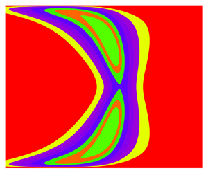
Figure 1 shows ${\lambda _y}({\boldsymbol {k}},y)$ for the turbulent channel flows at ${Re_\tau } = 180$ and $550$, where the wavenumber vector ${\boldsymbol {k}}h = (2,4)$ represents large-scale structures, and $Re_{\tau}=u_{\tau}h{/}\nu$ is the Reynolds number based on the friction velocity $u_{\tau}$, with h being the half-height of the channel. We use the semicircle function to fit the wall-normal distribution of ${\lambda _y}({\boldsymbol {k}},y)$:

(3.21)\begin{equation} {\lambda _y}({\boldsymbol{k}},y) = \beta ({\boldsymbol{k}})\,\sqrt {{h^2} - {y^2}}, \end{equation}

where $\beta ({\boldsymbol {k}})$ is determined to minimize the error $\int _{- h}^h {{{[\lambda _y^{DNS}({\boldsymbol {k}},y) - \beta ({\boldsymbol {k}})\sqrt {{h^2} - {y^2}} ]}^2}\,{{\rm d} y}}$. That is,

(3.22)\begin{equation} \beta ({\boldsymbol{k}}) = \frac{{\displaystyle\int_{ - h}^h {\lambda _y^{DNS}({\boldsymbol{k}},y)\,\sqrt {{h^2} - {y^2}} \,{{\rm d}y}}}}{{\displaystyle\int_{ - h}^h {({h^2} - {y^2})\,{{\rm d} y}}}}, \end{equation}

where $\lambda _y^{DNS}({\boldsymbol {k}},y)$ is the result obtained from (3.20) through DNS data. For the wavenumber vector ${\boldsymbol {k}}h = (2,4)$, $\beta ({\boldsymbol {k}}) = 0.075$ at ${Re_\tau } = 180$, and $\beta ({\boldsymbol {k}}) = 0.046$ at ${Re_\tau } = 550$. In this paper, $\beta ({\boldsymbol {k}})$ is determined from (3.22) using DNS data. The numerical examination shows that the results are not sensitive to the parameter ${\lambda _y}({\boldsymbol {k}},y)$. In fact, the constant ${\lambda _y}({\boldsymbol {k}},y) = 0.045h$ leads to results similar to those obtained from (3.21) and (3.22).

Figure 1. Characteristic length scale ${\lambda _{y}}({\boldsymbol {k}},y)$ of the turbulent channel flows at ${\boldsymbol {k}}h = (2,4)$ for large-scale structures. (a) Plots for ${Re_\tau } = 180$, where the red solid line shows the DNS result, and the blue dashed line shows $0.075\sqrt {{h^2} - {y^2}}$. (b) Plots for ${Re_\tau } = 550$, where the red solid line shows the DNS result, and the blue dashed line shows $0.046\sqrt {{h^2} - {y^2}}$.

Finally, we substitute the model (3.8) for nonlinear forcing into the governing equation (3.3) for resolvent analysis, and take the temporal Fourier transform of the resultant equation, giving the space–time Fourier mode ${\tilde {\boldsymbol u}}$ of velocity fluctuation as

(3.23)\begin{equation} {\tilde{\boldsymbol u}} = {{\boldsymbol{R}}_s}{\tilde{\boldsymbol f}}. \end{equation}

The operator ${{\boldsymbol {R}}_s}$ is given by

(3.24) $$\begin{gather} {{\boldsymbol{R}}_s} = {{\boldsymbol{B}}^{\rm T}}{\left( { - {\rm{i}}\omega \left[\begin{array}{@{}l@{}c@{}} {\boldsymbol{I}}\vphantom{{{\hat{\boldsymbol{\nabla}}}^{\rm T}}} & \\ & 0 \vphantom{{{\hat{\boldsymbol{\nabla}}}^{\rm T}}}\end{array}\right] - \left[\begin{array}{cc} {{{\boldsymbol{L}}_s}} & {- \hat{\boldsymbol{\nabla}}} \\ {- {{\hat{\boldsymbol{\nabla}}}^{\rm T}}} & 0 \end{array}\right]} \right)^{{-}1}}{\boldsymbol{B}}, \end{gather}$$

(3.25)$$\begin{gather}{{\boldsymbol{L}}_s} = \left[\begin{array}{ccc} { - {\rm{i}}{k_x}U + \nu\,{\hat{\nabla}^2} + {D_s}} & { - U'} & 0 \\ 0 & { - {\rm{i}}{k_x}U + \nu\,{\hat{\nabla}^2} + {D_s}} & 0 \\ 0 & 0 & { - {\rm{i}}{k_x}U + \nu\,{\hat{\nabla}^2} + {D_s}} \end{array}\right], \end{gather}$$

(3.26)$$\begin{gather}{D_s} ={-} \sqrt {k_x^2\,V_x^2(y) + k_z^2\,V_z^2(y)} + {\lambda_{y}}({\boldsymbol{k}},y)\,{\partial _y}({{V_y}(y)\,{\partial _y}}). \end{gather}$$

The operator ${{\boldsymbol {R}}_s}$ is called the sweeping-enhanced resolvent, analogous to the sweeping-enhanced transfer function ${R_s}$ in the DAR model. In fact, it is the conventional resolvent operator augmented by the eddy damping term that appears on the diagonal of matrix ${{\boldsymbol {L}}_s}$. In § 3.3, we discuss the difference between the sweeping-enhanced resolvent and the eddy-viscosity-enhanced resolvent. Therefore, the space–time cross-spectrum of velocity fluctuations is given by

(3.27)\begin{equation} {{\boldsymbol{\varPhi}}_{{\tilde{\boldsymbol u}\tilde{\boldsymbol u}}}} = {{\boldsymbol{R}}_s}{{\boldsymbol{\varPhi }}_{{\tilde{\boldsymbol f}\tilde{\boldsymbol f}}}} {\boldsymbol{R}}_s^*, \end{equation}

where ${{\boldsymbol {\varPhi }}_{{\tilde {\boldsymbol u}\tilde {\boldsymbol u}}}} = \langle {\tilde {\boldsymbol u}}({\boldsymbol {k}},\omega,y)\,{{\tilde {\boldsymbol u}}^ * }({\boldsymbol {k}},\omega,y')\rangle$ is the space–time cross-spectrum of velocity fluctuations, and ${{\boldsymbol {\varPhi } }_{{\tilde {\boldsymbol f}\tilde {\boldsymbol f}}}} = \langle {\tilde {\boldsymbol f}}({\boldsymbol {k}},\omega,y)\,{{\tilde {\boldsymbol f}}^ * }({\boldsymbol {k}},\omega,y')\rangle$ is the space–time cross-spectrum of nonlinear forcing.

3.2. Composition of the resolvents

By analogy to (2.7) in the DAR model, the sweeping-enhanced resolvent ${{\boldsymbol {R}}_s}$ defined in (3.24) is applied to white-in-time random forcing ${{\tilde {\boldsymbol f}}_t}$, yielding an intermediate random forcing ${\tilde {\boldsymbol f}}$ of finite correlation time

(3.28)\begin{equation} {\tilde{\boldsymbol f}} = {{\boldsymbol{R}}_s}{{\tilde{\boldsymbol f}}_t}. \end{equation}

Subsequently, the obtained random forcing ${\tilde {\boldsymbol f}}$ is used as the input to the same sweeping-enhanced resolvent as that in (3.28), leading to

(3.29)\begin{equation} {\tilde{\boldsymbol u}} = {{\boldsymbol{R}}_s}{\tilde{\boldsymbol f}}. \end{equation}

Therefore, the velocity fluctuation ${\tilde {\boldsymbol u}}$ is determined by the random forcing ${{\tilde {\boldsymbol f}}_t}$ through the composition of the sweeping-enhanced resolvent ${{\boldsymbol {R}}_s}$, that is,

(3.30)\begin{equation} {\tilde{\boldsymbol u}} = {\boldsymbol{R}}_s^2{{\tilde{\boldsymbol f}}_t}. \end{equation}

It follows that the space–time cross-spectrum of velocity fluctuations is given by

(3.31)\begin{equation} {{\boldsymbol{\varPhi }}_{{\tilde{\boldsymbol u}\tilde{\boldsymbol u}}}} = {\boldsymbol{R}}_s^2 {{\boldsymbol{\varPhi }}_{{{{\tilde{\boldsymbol f}}}_t}{{{\tilde{\boldsymbol f}}}_t}}}{\boldsymbol{R}}_s^{ * 2}, \end{equation}

where ${{\boldsymbol {\varPhi }}_{{{{\tilde {\boldsymbol f}}}_t}{{{\tilde {\boldsymbol f}}}_t}}} = \langle {{\tilde {\boldsymbol f}}_t}({\boldsymbol {k}},\omega,y)\,{\tilde {\boldsymbol f}}_t^ * ({\boldsymbol {k}},\omega,y')\rangle$ is the space–time cross-spectrum of the white-in-time random forcing ${{\tilde {\boldsymbol f}}_t}$. It is observed from (3.30) and (3.31) that the output and input are related by the composition of the sweeping-enhanced resolvent, ${\boldsymbol {R}}_s^2$. Accordingly, this composite resolvent is referred to as the ${\boldsymbol {R}}_s^2$ model.

The space–time cross-spectrum ${{\boldsymbol {\varPhi }}_{{{{\tilde {\boldsymbol f}}}_t}{{{\tilde {\boldsymbol f}}}_t}}}$ of the random forcing ${{\tilde {\boldsymbol f}}_t}$ is calculated from

(3.32)\begin{equation} {{\boldsymbol{\varPhi }}_{{{{\tilde{\boldsymbol f}}}_t}{{{\tilde{\boldsymbol f}}}_t}}}({\boldsymbol{k}},\omega ,y,y') = {\boldsymbol{I}}{[k_x^2\,V_x^2(y) + k_z^2\,V_z^2(y)]^{3/2}}\langle {v^2}(y)\rangle\,\delta (y - y'). \end{equation}

The space–time cross-spectrum depends on the variance of the wall-normal velocity fluctuations $\langle {v^2}(y)\rangle$ but is independent of the variances of streamwise and spanwise velocity fluctuations, $\langle {u^2}(y)\rangle$ and $\langle {w^2}(y)\rangle$. In fact, the wall-normal velocity fluctuations depend only on external forcing, as described by the Orr–Sommerfeld equation. However, the streamwise and spanwise velocity fluctuations depend on the wall-normal vorticity. According to the Squire equation, the wall-normal vorticity depends not only on external forcing but also on the energy production due to mean shear. The latter can be taken into account by the resolvent. Note that while the DAR model needs the spatial energy spectra of streamwise velocity fluctuations, the present ${\boldsymbol {R}}_s^2$ model needs only the variances of the velocity fluctuations. In the ${\boldsymbol {R}}_s^2$ model, the mean velocity $U(y)$, the r.m.s. of the velocity fluctuations $\sqrt {\langle {u^2}(y)\rangle }$, $\sqrt {\langle {v^2}(y)\rangle }$ and $\sqrt {\langle {w^2}(y)\rangle }$, and the factor $\beta ({\boldsymbol {k}})$ are taken from the DNS data.

Finally, we justify that the resolvent used in (3.28) is the same as that used in (3.29). In fact, the nonlinear forcing is found to exhibit space–time structures similar to those in turbulent flows (Morra et al. Reference Morra, Nogueira, Cavalieri and Henningson2021; Nogueira et al. Reference Nogueira, Morra, Martini, Cavalieri and Henningson2021), such as the streamwise vortices that are reminiscent of the streamwise vortex structures of velocity fluctuations. A different resolvent can be introduced to replace that used in (3.28). This offers more flexibility but definitely increases the number of undetermined parameters.

3.3. Comparison of sweeping-enhanced and eddy-viscosity-enhanced resolvents

The sweeping-enhanced resolvent is proposed in terms of the decorrelation process with the aim of predicting the space–time energy spectra. However, the eddy-viscosity-enhanced resolvent is based mainly on energy transfer. Although it is not yet used to predict space–time energy spectra, the eddy-viscosity-enhanced resolvent successfully reproduces the amplifications of coherent streaks and linear non-normal energy (Hwang & Cossu Reference Hwang and Cossu2010a,Reference Hwang and Cossub) and predicts the spatial energy spectra in the streamwise and spanwise directions (Gupta et al. Reference Gupta, Madhusudanan, Wan, Illingworth and Juniper2021). In fact, Hwang & Cossu (Reference Hwang and Cossu2010a,Reference Hwang and Cossub) introduced the eddy viscosity ${\nu _t}$ and random forcing ${\boldsymbol {f}}$ to represent the energy dissipation and extraction in the nonlinear forcing ${\boldsymbol {F}}$, leading to

(3.33)\begin{equation} {\boldsymbol{F}} = \boldsymbol{\nabla} {\boldsymbol{\cdot}} [{\nu _t}(\boldsymbol{\nabla} {\boldsymbol{u}} + \boldsymbol{\nabla} {{\boldsymbol{u}}^{\rm T}})] + {\boldsymbol{f}}. \end{equation}

In turbulent channel flows, the Cess model is used widely for eddy viscosity. It should be noted that the eddy viscosity can also be calculated from the mean velocity and the Reynolds-averaged NS equations (Hwang & Cossu Reference Hwang and Cossu2010a). The Cess model is written as

(3.34)\begin{equation} {\nu _t}(y) = \frac{\nu}{2}\sqrt{1 + \frac{{\kappa ^2}\,{Re}_\tau^2}{9} {{\left({1 - \frac{{{y^2}} }{{{h^2}}}} \right)}^2}{{\left({1 + \frac{{2{y^2}}}{{{h^2}}}}\right)}^2}{{(1-{\exp({-{y^+}/A})})}^2}} - \frac{\nu}{2}, \end{equation}

where $\kappa = 0.426$ is the Kármán constant, $A$ is a constant with $A = 25.4$, $y \in [ - h,h]$ is the wall-normal location, and ${y^ + } = {Re_\tau }(1 - |y|/h)$. The eddy viscosity in the Cess model is independent of the length scales of turbulent eddies.

Gupta et al. (Reference Gupta, Madhusudanan, Wan, Illingworth and Juniper2021) proposed that the eddy viscosity should depend on the length scales of turbulent eddies as

(3.35)$$\begin{gather} {\nu _t}(\lambda,y) = \frac{\lambda } {{\lambda + {\lambda _m}(y)}}\,{\nu _t}(y), \end{gather}$$

(3.36)$$\begin{gather}\frac{{{\lambda _m}(y)} } {h} = \frac{{50}}{{{{Re}_\tau }}} + \left( {2 -\frac{{50}}{{{{Re}_\tau }}}} \right)\tanh \left[{6\left( {1 - \frac{{|y|}}{h}} \right)} \right], \end{gather}$$

where $\lambda = 2{\rm \pi} /\sqrt {k_x^2 + k_z^2}$ is the wavelength. Here, ${\nu _t}(\lambda,y)$ becomes ${\nu _t}(y)$ for sufficiently large wavelengths $\lambda \to \infty$, and ${ \nu _t}(\lambda,y)$ becomes zero for sufficiently small wavelengths $\lambda \to 0$.

Taking the spatial ($x$–$z$) Fourier transform of (3.33), we obtain the spatial Fourier mode ${\hat {\boldsymbol F}}$ of the nonlinear forcing. Then substituting ${\hat {\boldsymbol F}}$ into (3.3) and taking the temporal Fourier transform of (3.3) leads to the space–time Fourier mode ${\tilde {\boldsymbol u}}$ of the velocity fluctuations:

(3.37)\begin{equation} {\tilde{\boldsymbol u}} = {{\boldsymbol{R}}_{{\nu _t}}}\,{\tilde{\boldsymbol f}}, \end{equation}

where ${{\boldsymbol {R}}_{{\nu _t}}}$ is referred to as the ${\nu _t}$-enhanced resolvent that is given by

(3.38) $$\begin{gather} {{\boldsymbol{R}}_{{\nu _t}}} = {{\boldsymbol{B}}^{\rm T}}{\left( { - {\rm{i}}\omega \left[ \begin{array}{@{}cc@{}} {\boldsymbol{I}}\vphantom{{{\hat{\boldsymbol{\nabla}}}^{\rm T}}} & \\ & 0\vphantom{{{\hat{\boldsymbol{\nabla}}}^{\rm T}}} \end{array}\right] - \left[\begin{array}{@{}cc@{}} {{{\boldsymbol{L}}_{{\nu _t}}}} & { -\hat{\boldsymbol{\nabla}}} \\ {- {{\hat{\boldsymbol{\nabla}}}^{\rm T}}} & 0 \end{array}\right]}\right)^{ - 1}}{\boldsymbol{B}}, \end{gather}$$

(3.39)$$\begin{gather}{\small {{\boldsymbol{L}}_{{\nu _t}}} = \left[ \begin{array}{@{}ccc@{}} { - {\rm{i}}{k_x}U + {\nu _T}{\hat{\nabla}^2} + {\nu'_T}{\partial _y}} & { - U' + {\rm{i}}{k_x}{\nu'_T}} & 0 \\ 0 & { - {\rm{i}}{k_x}U + {\nu _T}{\hat{\nabla}^2} + 2{\nu'_T}{\partial _y}} & 0 \\ 0 & {{\rm{i}}{k_z}{\nu'_T}} & { - {\rm{i}}{k_x}U + {\nu _T}{\hat{\nabla}^2} + {\nu'_T}{\partial _y}} \end{array}\right],} \end{gather}$$

with ${\nu _T} = \nu + {\nu _t}$. Note that the ${\nu _t}$-enhanced resolvent ${{\boldsymbol {R}}_{{\nu _t}}}$ in (3.38) with ${\nu _t} = 0$ becomes the resolvent ${\boldsymbol {R}}$ in (3.7). Therefore, the space–time cross-spectrum of the velocity is

(3.40)\begin{equation} {{\boldsymbol{\varPhi }}_{{\tilde{\boldsymbol u}\tilde{\boldsymbol u}}}} = {{\boldsymbol{R}}_{{\nu _t}}}{{\boldsymbol{\varPhi }}_{{\tilde{\boldsymbol f}\tilde{\boldsymbol f}}}}{\boldsymbol{R}}_{{\nu _t}}^*. \end{equation}

In LNSEs and resolvent-based methods, white forcing is used widely (Farrell & Ioannou Reference Farrell and Ioannou1998; Bamieh & Dahleh Reference Bamieh and Dahleh2001; Jovanović & Bamieh Reference Jovanović and Bamieh2005; Liu & Gayme Reference Liu and Gayme2020; Gupta et al. Reference Gupta, Madhusudanan, Wan, Illingworth and Juniper2021). The forcing intensity is usually taken as constant in the wall-normal direction (Morra et al. Reference Morra, Semeraro, Henningson and Cossu2019):

(3.41)\begin{equation} {{\boldsymbol{\varPhi}}_{{\tilde{\boldsymbol f}\tilde{\boldsymbol f}}}}({\boldsymbol{k}},\omega ,y,y') = {\boldsymbol{I}}\,\delta (y - y'), \end{equation}

which is used in the B model (see § 4).

Gupta et al. (Reference Gupta, Madhusudanan, Wan, Illingworth and Juniper2021) further proposed that the forcing intensity depends on the eddy viscosity as

(3.42)\begin{equation} {{\boldsymbol{\varPhi }}_{{\tilde{\boldsymbol f}\tilde{\boldsymbol f}}}}({\boldsymbol{k}},\omega,y,y') = {\boldsymbol{I}}\,\nu _t^2(y)\,\delta (y - y'), \end{equation}

where the Cess model is used for ${\nu _t}$. The forcing spectra in (3.42) are used in the W model (see § 4). Similarly, the Cess model can be replaced by the wavelength-dependent eddy viscosity (3.35) and (3.36), giving

(3.43)\begin{equation} {{\boldsymbol{\varPhi }}_{{\tilde{\boldsymbol f}\tilde{\boldsymbol f}}}}({\boldsymbol{k}},\omega ,y,y') = {\boldsymbol{I}}\,\nu _t^2(\lambda ,y)\,\delta (y - y'). \end{equation}

The forcing spectra in (3.43) are used in the $\lambda$ model (see § 4).

Therefore, both eddy viscosity and random forcing depend not only on the wall-normal locations but also on the wavenumbers. Consequently, the $\lambda$ model proposed by Gupta et al. (Reference Gupta, Madhusudanan, Wan, Illingworth and Juniper2021) with ${\nu _t}(\lambda,y)$ and the wall-distance dependence of the forcing intensity accounts for the energy transfer along the wall-normal direction, and the energy transfer between different length scales in space. Therefore, this model correctly predicts the two-dimensional spatial spectra. However, this cannot ensure the correct prediction of frequency spectra and time correlations.

The eddy viscosity and sweeping velocity lead to different characteristic decay times, as shown in figures 7 and 8, while both give rise to temporal decorrelation of coherent structures. In fact, as the wall distance increases, the eddy viscosity in the logarithmic region becomes larger and thus gives rise to smaller characteristic decay time scales. This is in contrast to the decorrelation process in turbulent channel flows, where the characteristic decay time scales become larger with increasing wall distance. It is noted in (3.34) that the eddy viscosity in the logarithmic region is ${\nu _t}(y) = {u_\tau }\kappa d$, where the wall distance is given by $d = 1 - |y|/h$, and $\kappa d$ is the mixing length. However, as the wall distance increases, the sweeping velocities decrease and thus give rise to larger characteristic decay time scales. This is consistent with the observation that the time correlations in turbulent channel flows decay more slowly with increasing wall distance.

Van Atta & Wyngaard (Reference Van Atta and Wyngaard1975) pointed out that the high-order spectra are related to the energy spectra of velocity fluctuations through the random sweeping velocity. This result was justified theoretically and validated by Praskovsky et al. (Reference Praskovsky, Gledzer, Karyakin and Zhou1993), Katul et al. (Reference Katul, Banerjee, Cava, Germano and Porporato2016) and Huang & Katul (Reference Huang and Katul2022). Note that the spectra of nonlinear forcing are the fourth-order moments of velocity fluctuations, and the energy spectra are the second-order moments of velocity fluctuations. Therefore, the spectra of nonlinear forcing are related to the velocity spectra through the random sweeping velocity, supporting the sweeping-enhanced resolvent in the present study.

4. Numerical results

Two sets of DNS of turbulent channel flows at ${{{Re}}_\tau }= 180$ and $550$ are performed in this work. The NS equations are solved using a pseudo-spectral method with a $3/2$ de-aliasing rule. Periodic boundary conditions are applied in the streamwise and spanwise directions, and no-slip conditions are applied at the walls. For the case ${{{Re}}_\tau } = 180$, the computational domain is $8{\rm \pi} h \times 2h \times 4{\rm \pi} h$ in the streamwise ($x$), wall-normal ($y$) and spanwise ($z$) directions. The $384 \times 128 \times 384$ grid is used. The time step is $5 \times {10^{ - 3}}h/{U_b}$, where ${U_b}$ is the bulk velocity. In the statistically stationary state, the instantaneous flow fields are stored every 10 steps, and a total of 5000 steps are stored. For the case ${{{Re}}_\tau } = 550$, the computational domain is $4{\rm \pi} h \times 2h \times 2{\rm \pi} h$ in the streamwise, wall-normal and spanwise directions, respectively. The $576 \times 256 \times 576$ grid is used. The time step is $1 \times {10^{-3}}h/{U_b}$. In the statistically stationary state, the instantaneous flow fields are stored every 50 steps, and a total of 5400 steps are stored. The NS solver and dataset have been validated in previous studies (Wu et al. Reference Wu, Geng, Yao, Xu and He2017; Wu & He Reference Wu and He2020, Reference Wu and He2021b).

To perform the temporal Fourier transform, the Hanning window is used with a $50\,\%$ overlap and window length $51.2h/{U_b}$. The spanwise length scale of large-scale structures in wall turbulence is ${\lambda _z} \approx h\unicode{x2013}1.5h$, and the streamwise length scale is ${\lambda _x} \approx 2{\lambda _z}$ (Kim & Adrian Reference Kim and Adrian1999; Smits, McKeon & Marusic Reference Smits, McKeon and Marusic2011; Morra et al. Reference Morra, Semeraro, Henningson and Cossu2019). Therefore, the wavenumber range of large-scale structures is ${k_z}h = 2{\rm \pi} h/{\lambda _z} \approx 4\unicode{x2013}6$ and ${k_x} \approx {k_z}/2$. In this paper, the wavenumber vector $({k_x}h,{k_z}h) = (2,4)$ is taken for the analysis of the large-scale structures.

Five resolvent-based models are used in this work, and the settings (i.e. resolvent and forcing spectra) of these models are shown in table 1. The model with neither eddy viscosity nor sweeping is referred to as the $\nu$ model (Morra et al. Reference Morra, Semeraro, Henningson and Cossu2019), and the three models with eddy viscosity are referred to as the B model, W model and $\lambda$ model (Gupta et al. Reference Gupta, Madhusudanan, Wan, Illingworth and Juniper2021). We use the following symbols for the eddy-viscosity-enhanced models in Gupta et al. (Reference Gupta, Madhusudanan, Wan, Illingworth and Juniper2021): ‘B’ in the B model refers to baseline, where the forcing spectrum is uniform in the wall-normal direction; ‘W’ in the W model refers to wall-distance dependence, where the forcing spectrum depends on the wall distance; and ‘$\lambda$’ in the $\lambda$ model indicates that the eddy viscosity and forcing spectrum depend on the wavelength $\lambda$. The ${\boldsymbol {R}}_s^2$ model refers to the proposed model in this paper. In the following, we use these models to predict the space–time statistics of the large-scale structures in turbulent channel flows, and compare these predictions with the DNS results.

Table 1. Summary of the resolvent-based models used in the present study.

The space–time energy spectrum, or one-point wavenumber–frequency spectrum, of the streamwise velocity fluctuation is expressed as

(4.1)\begin{equation} \varPhi ({\boldsymbol{k}},\omega ,y) = \langle \tilde u({\boldsymbol{k}},\omega ,y)\,{\tilde u^ * }({\boldsymbol{k}},\omega ,y)\rangle, \end{equation}

where $\tilde u({\boldsymbol {k}},\omega,y)$ is the space–time Fourier mode of the streamwise velocity fluctuation. The space–time cross-spectrum, or two-point wavenumber–frequency cross-spectrum, of the streamwise velocity fluctuation is expressed as

(4.2)\begin{equation} \varPhi ({\boldsymbol{k}},\omega ,y,y') = \langle \tilde u({\boldsymbol{k}},\omega ,y)\, {{\tilde u}^ * }({\boldsymbol{k}},\omega ,y')\rangle. \end{equation}

In the numerical calculation, ${\tilde {\boldsymbol u}}$ is a column vector of size $3N$, given by

(4.3)\begin{align} {\tilde{\boldsymbol u}} &= \left[\tilde u({y_1}),\ldots,\tilde u({y_i}),\ldots, \tilde u({y_N}),\tilde v({y_1}),\ldots,\tilde v({y_i}),\ldots,\tilde v({y_N}), \right.\nonumber\\ &\quad \left.\tilde w({y_1}),\ldots,\tilde w({y_i}),\ldots, \tilde w({y_N})\right]^{\rm T}, \end{align}

where ${y_i}$ is the wall-normal coordinate of the $i$th grid point ($i = 1,\ldots,N$), $N$ is the number of wall-normal grid points, and $3$ denotes the number of velocity components; ${{\boldsymbol {\varPhi }}_{{\tilde {\boldsymbol u}\tilde {\boldsymbol u}}}}$ in (3.31) and (3.40) is a matrix of size $3N \times 3N$. In the matrix ${{\boldsymbol {\varPhi }}_{{\tilde {\boldsymbol u}\tilde {\boldsymbol u}}}}$, the ${(i,j)}$th element represents the space–time cross-spectrum $\varPhi ({\boldsymbol {k}},\omega,{y_i},{y_j})$, and the ${(i,i)}$th element represents the space–time energy spectrum $\varPhi ({\boldsymbol {k}},\omega,{y_i})$.

We focus on the streamwise velocity spectral distribution in the frequency ($\omega$) and wall-normal ($y$) directions. Integrating the space–time energy spectrum over $\omega$ and $y$, we obtain the total streamwise velocity energy

(4.4)\begin{equation} {\varPhi _I}({\boldsymbol{k}}) = \int_{ - h}^h {{{\rm d} y}\int_{ - \infty }^\infty {{\rm d}\omega\, \varPhi ({\boldsymbol{k}},\omega ,y)}}, \end{equation}

which is used as the normalization factor to obtain the streamwise velocity spectral distribution. We note that the spectral distributions from the DNS and those models are normalized by their corresponding integrated spectrum in (4.4).

Figures 2 and 3 plot the frequency spectral distributions in the wall-normal direction, $\varPhi ({\boldsymbol {k}},\omega,y)/{\varPhi _I}({\boldsymbol {k}})$, at ${\boldsymbol {k}}h = (2,4)$ for large-scale structures at the two Reynolds numbers ${Re_\tau } = 180$ and $550$, respectively. The ${\boldsymbol {R}}_s^2$ model reproduces the curved ribbon region in the DNS, in which the coloured contours of the same levels have similar locations, areas and shapes. The red-ribbon region of the largest level in the $\nu$ model is relatively narrow, as was also observed by Morra et al. (Reference Morra, Semeraro, Henningson and Cossu2019). The regions of coloured ribbons in the B model, the W model and the $\lambda$ model are spread over broader ranges of frequencies compared to the DNS results because the eddy viscosity gives rise to smaller decorrelation time scales and thus larger energy-contained frequencies. In particular, the red ribbons in the B model are concentrated in the near-wall region because the eddy viscosities used in this model are incorrectly larger in the outer-layer region and smaller in the near-wall region. The forcing intensity used in the W model depends on the wall-normal locations, balancing the effect of the eddy viscosity dependent on the wall-normal locations, and leading to red and yellow regions that are similar to those for the DNS results. However, the eddy viscosity in the $\lambda$ model is smaller than that in the W model and thus reduces the extent of the ribbon-like frequency regions. We note that both the sweeping term and the forcing intensity in the ${\boldsymbol {R}}_s^2$ model depend on the wall-normal locations and characteristic length scales of the turbulent eddies, and that the frequency spectral distribution in the wall-normal direction is consistent with that for the DNS results.

Figure 2. Frequency spectral distributions in the wall-normal direction, $\varPhi ({\boldsymbol {k}},\omega,y)/{\varPhi _I}({\boldsymbol {k}})$, at ${\boldsymbol {k}}h = (2,4)$ for large-scale structures at $Re_\tau = 180$: (a) DNS, (b) $\nu$ model, (c) B model, (d) W model, (e) $\lambda$ model, ( f) ${\boldsymbol {R}}_s^2$ model.

Figure 3. Frequency spectral distributions in the wall-normal direction, $\varPhi ({\boldsymbol {k}},\omega,y)/{\varPhi _I}({\boldsymbol {k}})$, at ${\boldsymbol {k}}h = (2,4)$ for large-scale structures at ${Re_\tau } = 550$: (a) DNS, (b) $\nu$ model, (c) B model, (d) W model, (e) $\lambda$ model, ( f) ${\boldsymbol {R}}_s^2$ model.

The differences between the space–time energy spectra obtained by the above models and by the DNS can be quantified using the Hellinger distance (Wu & He Reference Wu and He2020, Reference Wu and He2021b) that is defined as

(4.5)\begin{equation} {d_H}({\boldsymbol{k}},y) = {\left[ {\int {{{\left({\sqrt{\frac{{{\varPhi^{{model}}} ({\boldsymbol{k}},\omega ,y)}}{{{\varPhi^{{model}}}({\boldsymbol{k}},y)}}} - \sqrt{\frac{{{\varPhi ^{{{DNS}}}}({\boldsymbol{k}},\omega ,y)}} {{{\varPhi^{{{DNS}}}}({\boldsymbol{k}},y)}}} } \right)}^2}{\rm d}\omega } } \right]^{1/2}}. \end{equation}

Figure 4 shows the Hellinger distance ${d_H}({\boldsymbol {k}},y)$ at ${\boldsymbol {k}}h = (2,4)$ for large-scale structures. The Hellinger distances between the $\nu$ model and the DNS results are the largest. In the near-wall region, the Hellinger distances from the W model, $\lambda$ model and ${\boldsymbol {R}}_s^2$ model are similar. However, in most regions of the channel, the Hellinger distances from the ${\boldsymbol {R}}_s^2$ model are significantly smaller than those from other models, implying that the ${\boldsymbol {R}}_s^2$ model is more consistent with the DNS results.

Figure 4. Hellinger distance ${d_H}({\boldsymbol {k}},y)$ at ${\boldsymbol {k}}h = (2,4)$ for large-scale structures: (a) ${Re_\tau } = 180$, (b) ${Re_\tau } = 550$.

The resolvent models are examined in terms of the time correlations of the spatial Fourier modes at a fixed wavenumber and one wall-normal location that are given by

(4.6)\begin{equation} R({\boldsymbol{k}},\tau ,y) = \frac{{\displaystyle\int_{-\infty}^\infty {\varPhi ({\boldsymbol{k}},\omega ,y)\exp({-{\rm i}\omega\tau})\,{\rm d}\omega}}}{{\displaystyle\int_{-\infty}^\infty {\varPhi ({\boldsymbol{k}},\omega ,y)\,{\rm d}\omega}}}. \end{equation}

Figures 5 and 6 show the time correlations $|R({\boldsymbol {k}},\tau,y)|$ at ${\boldsymbol {k}}h = (2,4)$ for large-scale structures and at three wall-normal locations: ${y^ + } = 5$, $50$ and $180$ for ${Re_\tau } = 180$, and ${y^+} = 5$, $92$ and $550$ for ${Re_\tau } = 550$. The time correlations in the two cases exhibit consistent decay behaviours. Accordingly, we discuss only the case for ${Re_\tau } = 550$. It is observed from the DNS that the time correlation at ${y^+} = 92$ decays more rapidly than that at ${y^+} = 550$, while the time correlation at ${y^+} = 5$ shows the fastest decays. The ${\boldsymbol {R}}_s^2$ model reproduces the DNS results, where the decay becomes slower with increasing wall-normal distance. However, the resolvent model without eddy viscosity ($\nu$ model) and the eddy-viscosity-enhanced models (B model, W model and $\lambda$ model) give decay behaviours that are inconsistent with the DNS results, where the time correlations at ${y^ + } = 92$ decay more slowly than those at ${y^ + } = 550$. Furthermore, due to the composition of the sweeping-enhanced resolvent, the time correlations in figure 6( f) gradually decrease over a short time, which is in agreement with the DNS results. However, the time correlations obtained from the $\nu$ model, B model, W model and $\lambda$ model fall steeply at short times since the white-in-time external forcing acts on the velocity modes and thus leads to vanishing Taylor time microscales.

Figure 5. Amplitude of the time correlations $|R({\boldsymbol {k}},\tau,y)|$ at ${\boldsymbol {k}}h = (2,4)$ for large-scale structures and at three wall-normal locations at ${Re_\tau } = 180$. Red solid lines, ${y^ + } = 180$; blue dashed lines, ${y^ + } = 50$; brown dash-dotted lines, ${y^ + } = 5$. (a) DNS, (b) $\nu$ model, (c) B model, (d) W model, (e) $\lambda$ model, ( f) ${\boldsymbol {R}}_s^2$ model.

Figure 6. Amplitude of the time correlations $|R({\boldsymbol {k}},\tau,y)|$ at ${\boldsymbol {k}}h = (2,4)$ for large-scale structures and at three wall-normal locations at ${Re_\tau } = 550$. Red solid lines, ${y^ + } = 550$; blue dashed lines, ${y^ + } = 92$; brown dash-dotted lines, ${y^ + } = 5$. (a) DNS, (b) $\nu$ model, (c) B model, (d) W model, (e) $\lambda$ model, ( f) ${\boldsymbol {R}}_s^2$ model.

To quantify the short-time decay of the time correlations predicted by the resolvent models, we introduce the characteristic decay time scales as follows:

(4.7)\begin{equation} |R({\boldsymbol{k}},\tau = {T_d},y)| = {R_d}. \end{equation}

The characteristic decay time scale ${T_d}({\boldsymbol {k}},y)$ is that for which the time correlations decay to a certain value ${R_d}$, and describes the effects of white-in-time external forcing on time correlations. In this paper, we take ${R_d} = 0.9$. Different values of ${R_d}$ (e.g. ${R_d} = 0.95$ and $0.8$) are also taken, and the obtained results (not shown in this paper) do not change the conclusions.

Figures 7 and 8 compare the characteristic decay time scales obtained from the resolvent-based models and the DNS at ${\boldsymbol {k}}h = (2,4)$ for ${Re_\tau } = 180$ and $550$, respectively. To illustrate the necessity of composite resolvents, we compare the compositions of the resolvents, such as the ${\nu ^2}$ model, B$^2$ model, W$^2$ model, ${\lambda ^2}$ model and ${\boldsymbol {R}}_s^2$ model, with the resolvents themselves, the $\nu$ model, B model, W model, $\lambda$ model and ${{\boldsymbol {R}}_s}$ model. The characteristic time scales in the DNS increase with increasing wall distance. However, the characteristic time scales for the $\nu$ model are significantly larger than those for the DNS results. The eddy-viscosity-enhanced resolvent models, such as the B model, the W model and the $\lambda$ model, significantly underpredict the DNS results. Furthermore, the obtained time scales increase in the near-wall region and incorrectly decrease in other regions. In the outer region, the characteristic time scales of the ${{\boldsymbol {R}}_s}$ model increase with increasing wall distance, which is consistent with the DNS results. However, they are one order of magnitude smaller than the DNS results. The characteristic time scales of the composite resolvents are significantly larger than those of the single resolvents. Consequently, the ${\nu ^2}$ model yields larger characteristic time scales than those obtained using the $\nu$ model. The characteristic time scales of the B$^2$ model, W$^2$ model and ${\lambda ^2}$ model increase with increasing wall distance, which is consistent with the DNS results. Therefore, compared with eddy-viscosity-enhanced resolvents, their composite models improve the characteristic time scales. However, the characteristic time scales obtained from these models are larger than those obtained from the DNS. Since the eddy viscosity of the ${\lambda ^2}$ model is smaller than that of the W$^2$ model, the characteristic time scales from the ${\lambda ^2}$ model are between the results of the W$^2$ model and the results of the ${\nu ^2}$ model. The characteristic time scales obtained from the ${\boldsymbol {R}}_s^2$ model are in good agreement with the DNS results. In fact, the ${\boldsymbol {R}}_s^2$ model includes the three essential elements: LNSE, random sweeping and random forcing. Therefore, it can reproduce the time correlations in the central region where random sweeping is dominant, and the time correlations in the near-wall region where in addition to random sweeping the mean shear, molecular viscosity and pressure play important roles.

Figure 7. Comparison of the characteristic decay time scales obtained by the resolvent-based models with the DNS at ${\boldsymbol {k}}h = (2,4)$ for ${Re_\tau } = 180$. Red solid lines, the DNS results; blue dashed lines, the results of the (a) $\nu$ model, (b) B model, (c) W model, (d) $\lambda$ model, and (e) ${\boldsymbol {R}}_s$ model; brown dash-dotted lines, the results of the (a) ${\nu ^2}$ model, (b) B$^2$ model, (c) W$^2$ model, (d) ${\lambda ^2}$ model, and (e) ${\boldsymbol {R}}_s^2$ model. The inset in (e) shows an enlarged view of the result of the ${\boldsymbol {R}}_s$ model.

Figure 8. Comparison of the characteristic decay time scales obtained by the resolvent-based models with the DNS at ${\boldsymbol {k}}h = (2,4)$ for ${Re_\tau } = 550$. Red solid lines, the DNS results; blue dashed lines, the results of the (a) $\nu$ model, (b) B model, (c) W model, (d) $\lambda$ model, and (e) ${\boldsymbol {R}}_s$ model; brown dash-dotted lines, the results of the (a) ${\nu ^2}$ model, (b) B$^2$ model, (c) W$^2$ model, (d) ${\lambda ^2}$ model, and (e) ${\boldsymbol {R}}_s^2$ model. The inset in (e) shows an enlarged view of the result of the ${\boldsymbol {R}}_s$ model.

In addition to the wavenumber vector ${\boldsymbol {k}}h = (2,4)$, we calculate the frequency spectral distributions and characteristic time scales at ${\boldsymbol {k}}h = (1,2)$ and ${\boldsymbol {k}}h = (4,8)$ for large-scale structures. The results (see Appendix A) show that the frequency spectral distributions and wall-normal variation trends of the characteristic time scales obtained using the ${\boldsymbol {R}}_s^2$ model are consistent with the DNS results. We further calculate the characteristic time scales obtained from the resolvent-based models at ${\boldsymbol {k}}h = (2,4)$ for ${Re_\tau } = 1000$ (see Appendix B). The results are similar to those at ${Re_\tau } = 180$ and $550$, implying the applicability of the ${\boldsymbol {R}}_s^2$ model at higher Reynolds numbers. Although this paper focuses on the streamwise velocity fluctuations, we also calculate the frequency spectral distributions and characteristic time scales of the spanwise and wall-normal velocity fluctuations of the wavenumber vectors ${\boldsymbol {k}}h = (1,2)$, ${\boldsymbol {k}}h = (2,4)$ and ${\boldsymbol {k}}h = (4,8)$ (see Appendix C), and the results obtained from the ${\boldsymbol {R}}_s^2$ model are also consistent with the DNS results.

Figure 9 compares the Taylor time microscales obtained using the ${\boldsymbol {R}}_s^2$ model with the DNS results at ${\boldsymbol {k}}h = (2,4)$. According to Wu & He (Reference Wu and He2021b), the Taylor time microscales obtained by the direct imposition of white-in-time random forcing are zero. Due to the composition of resolvents, the ${\boldsymbol {R}}_s^2$ model can yield non-zero Taylor time microscales ${\lambda _T}({\boldsymbol {k}},y)$ of the time correlation $|R({\boldsymbol {k}},\tau,y)|$, where Taylor time microscale ${\lambda _T}({\boldsymbol {k}},y)$ is defined as

(4.8)\begin{equation} {\lambda _T}({\boldsymbol{k}},y) = {[{{- \left.(1/2)\partial_{\tau \tau }^2|R ({\boldsymbol{k}},\tau,y)|\right|_{\tau = 0}}}]^{ - 1/2}}. \end{equation}

The Taylor time microscales obtained by the ${\boldsymbol {R}}_s^2$ model are in good agreement with the DNS results, particularly at ${Re_\tau } = 550$.

Figure 9. Comparison of the Taylor time microscales ${\lambda _T}({\boldsymbol {k}},y)$ from the ${\boldsymbol {R}}_s^2$ model with the DNS results at ${\boldsymbol {k}}h = (2,4)$. Red solid lines, the DNS results; blue dashed lines, the results of the ${\boldsymbol {R}}_s^2$ model. Plots for (a) ${Re_\tau } = 180$, (b) ${Re_\tau } = 550$.

Figure 10 compares the integral time scales ${T_I}$ at ${\boldsymbol {k}}h = (2,4)$ for the ${\boldsymbol {R}}_s^2$ model with the DNS results. The integral time scale ${T_I}$ of the time correlation is defined as

(4.9)\begin{equation} {T_I} = \int_0^{{\tau _0}} {|R({\boldsymbol{k}},\tau ,y)|\,{\rm d}\tau}, \end{equation}

where ${\tau _0}$ is determined by $|R({\boldsymbol {k}},{\tau _0},y)| = 0.2$. Due to the limited number of samples, the time correlations $|R({\boldsymbol {k}},\tau,y)|$ of the DNS oscillate at large separations. Therefore, the upper limit of the integration in (4.9) is taken as ${\tau _0}$ for $|R({\boldsymbol {k}},{\tau _0},y)| = 0.2$. The results of the ${\boldsymbol {R}}_s^2$ model are close to those obtained by the DNS, with only slight differences.

Figure 10. Comparison of the integral time scales ${T_I}$ from the ${\boldsymbol {R}}_s^2$ model with the DNS results at ${\boldsymbol {k}}h = (2,4)$. Red solid lines, the DNS results; blue dashed lines, the results of the ${\boldsymbol {R}}_s^2$ model. Plots for (a) ${Re_\tau } = 180$, (b) ${Re_\tau } = 550$.

Figures 11 and 12 show the cross-spectral distribution $|\varPhi ({\boldsymbol {k}},{\omega _p},y,y')|/{\varPhi _I} ({\boldsymbol {k}})$ of the streamwise velocity modes at ${\boldsymbol {k}}h = (2,4)$ for large-scale structures, and the peak frequencies ${\omega _p}h/{U_b} = 2.1$ for ${Re_\tau } = 180$, and ${\omega _p}h/{U_b} = 2$ for ${Re_\tau } = 550$. It is noted that the cross-spectral distribution at the given wavenumber vector and frequency is the correlation of the space–time Fourier modes at two wall-normal positions. The peak frequency is determined by maximizing the total frequency spectral distribution at the given wavenumber:

(4.10)\begin{equation} {\varPhi _T}({\boldsymbol{k}},\omega ) = \frac{{\displaystyle\int_{ - h}^h {\varPhi ({\boldsymbol{k}},\omega ,y)\,{{\rm d} y}}}} {{{\varPhi _I}({\boldsymbol{k}})}} . \end{equation}

The cross-spectral distributions in the two Reynolds numbers exhibit similar behaviours. Accordingly, we discuss only the case for ${Re_\tau } = 550$. It is observed from the DNS that the cross-spectral distribution is maximal along the diagonal line $y = y'$ and decays most rapidly in the direction normal to the diagonal line. The ${\boldsymbol {R}}_s^2$ model reproduces the results observed for the DNS. In particular, it reproduces the coloured contours of different levels, namely their elliptical shapes and areas. The eddy-viscosity-enhanced model improves the predictions of the shapes and areas of coloured contours (see figures 12c,d)), and the gradual changes of the coloured contours (see figure 12e). However, the spectral peaks are underpredicted in figure 12(c) and overpredicted in figure 12(e). Note that the DAR model cannot predict the wall-normal two-point cross-spectra. However, the prediction of the cross-spectra can be achieved by the ${\boldsymbol {R}}_s^2$ model, where an LNSE is used to replace Taylor's frozen-flow model in the DAR model.

Figure 11. Amplitude of the cross-spectral distribution $|\varPhi ({\boldsymbol {k}},{\omega _p},y,y')|/{\varPhi _I} ({\boldsymbol {k}})$ of the streamwise velocity modes at ${\boldsymbol {k}}h = (2,4)$ for large-scale structures and the peak frequency ${\omega _p}h/{U_b} = 2.1$ for ${Re_\tau } = 180$: (a) DNS, (b) $\nu$ model, (c) B model, (d) W model, (e) $\lambda$ model, ( f) ${\boldsymbol {R}}_s^2$ model.

Figure 12. Amplitude of the cross-spectral distribution $|\varPhi ({\boldsymbol {k}},{\omega _p},y,y')|/{\varPhi _I} ({\boldsymbol {k}})$ of the streamwise velocity modes at ${\boldsymbol {k}}h = (2,4)$ for large-scale structures and the peak frequency ${\omega _p}h/{U_b} = 2$ for ${Re_\tau } = 550$: (a) DNS, (b) $\nu$ model, (c) B model, (d) W model, (e) $\lambda$ model, ( f) ${\boldsymbol {R}}_s^2$ model.

The differences in the cross-spectral distribution between the models and the DNS can be quantified using the function ${E_c}({\boldsymbol {k}},{\omega _p},y)$, defined as

(4.11)\begin{equation} {E_c}({\boldsymbol{k}},{\omega _p},y) = \int {\left|{\frac{{|{\varPhi^{{model}}}({\boldsymbol{k}},{\omega_p},y,y')|}}{{\varPhi _I^{{model}}({\boldsymbol{k}})}} - \frac{{|{\varPhi^{{{DNS}}}}({\boldsymbol{k}},{\omega _p},y,y')|}}{{\varPhi _I^{{{DNS}}} ({\boldsymbol{k}})}}}\right|{{\rm d} y}'}. \end{equation}

The function ${E_c}({\boldsymbol {k}},{\omega _p},y)$ measures the error in the cross-spectral distribution of the model relative to the DNS result. Figure 13 plots ${E_c}({\boldsymbol {k}},{\omega _p},y)$ of the different models at ${\boldsymbol {k}}h = (2,4)$. The error of the $\nu$ model is largest, and the errors for the W model and ${\boldsymbol {R}}_s^2$ model are smaller. At the peak of the cross-spectral distributions ($|y/h| \approx 0.63$), the error of the ${\boldsymbol {R}}_s^2$ model is smallest.

Figure 13. Errors ${E_c}({\boldsymbol {k}},{\omega _p},y)$ in the cross-spectral distributions obtained by different models relative to the DNS results at ${\boldsymbol {k}}h = (2,4)$: (a) ${Re_\tau } = 180$, (b) ${Re_\tau } = 550$. Two vertical lines are shown at $|y/h| = 0.63$ to indicate the peaks of the cross-spectral distributions.